<?xml version="1.0" encoding="utf-8"?><feed xmlns="http://www.w3.org/2005/Atom" xml:lang="en"><generator uri="https://jekyllrb.com/" version="4.4.1">Jekyll</generator><link href="https://cagrislist.org/feed.xml" rel="self" type="application/atom+xml" /><link href="https://cagrislist.org/" rel="alternate" type="text/html" hreflang="en" /><updated>2026-10-09T10:30:22+00:00</updated><id>https://cagrislist.org/feed.xml</id><title type="html">Çağrı Eser</title><subtitle>Personal website of Çağrı Eser</subtitle><author><name>Çağrı Eser</name></author><entry><title type="html">The n-dimensional Gaussian</title><link href="https://cagrislist.org/blog/2026/10/09/the-n-dimensional-gaussian/" rel="alternate" type="text/html" title="The n-dimensional Gaussian" /><published>2026-10-09T00:00:00+00:00</published><updated>2026-10-09T00:00:00+00:00</updated><id>https://cagrislist.org/blog/2026/10/09/the-n-dimensional-gaussian</id><content type="html" xml:base="https://cagrislist.org/blog/2026/10/09/the-n-dimensional-gaussian/"><![CDATA[<p class="callout"><small> This is the fourth entry in the
<a href="/blog/2026/09/16/a-leap-into-high-dimensional-space/">high-dimensional space blog series</a>.
</small></p>

<p>The normal distribution is everywhere in machine learning. Off of the top of my head, we use it for</p>

<ul>
  <li>Modeling measurement error and uncertainty (Gauss’s starting point)</li>
  <li>A popular choice for the prior of a latent distribution</li>
  <li>Sampling noise for methods such as autoencoders and GANs</li>
  <li>As a target distribution for learned representations, most recently seen in <a class="citation" href="#balestriero2025lejepa">(Balestriero &amp; LeCun, 2025)</a>.</li>
</ul>

<p>among many others. Our goal today is to look at the multivariate ($n$-dimensional) normal distribution in high-dimensional space.</p>

<h2 id="recalling-the-gaussian">Recalling the Gaussian</h2>

<p>The normal (or <em>Gaussian</em>) distribution $\mathcal{N}(x; \mu, \sigma^2)$ for $x \in \mathbb{R}$ is defined with the following probability density function in the single variable case:</p>

\[\mathcal{N}(x;\mu, \sigma^2) = \frac{1}{\sqrt{2\pi\sigma^2}}\exp\left\{-\frac{(x - \mu)^2}{2\sigma^2}\right\}.\]

<p>We usually drop the $x$ part and write $\mathcal{N}(\mu, \sigma^2)$.</p>

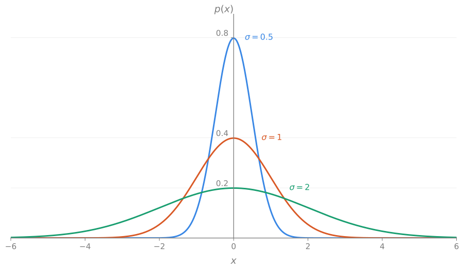
<p>Visually, we know it more commonly as the “bell curve”:</p>

<figure>
  <center>
  <img src="/assets/blog/high-dimensional-space/the-n-dimensional-gaussian/gaussians-1d.svg" alt="Simple 1D Gaussians." />
  <figcaption><small><i>Normal distributions $\mathcal{N}(0, \sigma^2)$ with varying standard deviation. </i></small></figcaption>
  </center>
</figure>

<p>Note that while the probability decreases exponentially with distance from the mean, the possible values for $x$ technically range from $-\infty$ to $\infty$.</p>

<div class="callout">

  <p>The normal distribution $\mathcal{N}(0, 1)$ with zero mean and unit variance is called the <em>standard normal distribution</em>.</p>

</div>

<hr />

<p>The normal distribution also has the corresponding cumulative distribution function (CDF), which is obtained by integrating the pdf from $-\infty$ to a target $x$:</p>

\[\Phi(x) = \frac{1}{\sqrt{2\pi}}\int_{-\infty}^{x}e^{-t^2/2}\,dt.\]
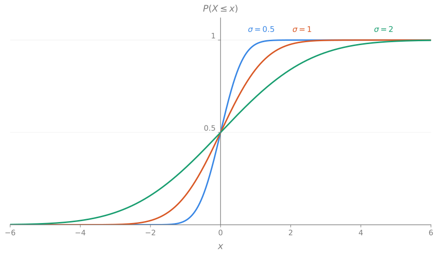
<figure>
  <center>
  <img src="/assets/blog/high-dimensional-space/the-n-dimensional-gaussian/gaussians-1d-cdf.svg" alt="CDF of Simple 1D Gaussians." />
  <figcaption><small><i>CDF of 1D Gaussians with varying standard deviation. </i></small></figcaption>
  </center>
</figure>

<p>As $\sigma$ increases the distribution becomes flatter, and as a result the CDF converges to $1$ more slowly. In the opposite direction, as $\sigma\to 0$ the peak of the PDF gets sharper until it becomes an infinitely tall spike on $x=\mu$ with total mass 1 (i.e., a <a href="https://en.wikipedia.org/wiki/Dirac_delta_function">Dirac delta function</a>), which produces a step function as the CDF.</p>

<div class="callout callout-note">

  <p>In general, a <strong>Gaussian function</strong> is a function $f$ in the form $f(x) = e^{-\alpha x^2}$. We saw functions of this form in our analysis of the $n$-ball and its corresponding boundary sphere, which indicates a preliminary connection between them and the Gaussian.</p>

</div>

<p>Given the historical context that we’ll uncover later in the article, from this point on I’ll refer to the distribution as the Gaussian.</p>

<h2 id="two-core-properties-of-the-gaussian">Two core properties of the Gaussian</h2>

<p>We briefly go over the two most “obvious” but crucial properties of the distribution.</p>

<ul>
  <li>
    <p>The mean of the Gaussian is $\mathbb{E}[X] = \mu$.</p>
  </li>
  <li>
    <p>The variance of the Gaussian is $\mathbb{V}[X] = \sigma^2$.</p>
  </li>
</ul>

<details class="callout callout-why">
  <summary><b>Why?</b></summary>

  <p>Let’s start with the mean. We have</p>

\[\mathbb{E}[X] = \int_{-\infty}^{\infty} x\,p(x)\,dx = \frac{1}{\sqrt{2\pi \sigma^2}}\int_{-\infty}^{\infty} x\,e^{-(x-\mu)^2/2\sigma^2}\,dx.\]

  <p>Let $u = (x - \mu)/\sigma$, with $du = (1/\sigma)\,dx$. Then</p>

\[\begin{align}
\mathbb{E}[X] &amp;= \frac{1}{\sqrt{2\pi\sigma^2}}\int_{-\infty}^{\infty} (\mu + \sigma\,u) \cdot e^{-u^2/2}\cdot \sigma\,du \\
  &amp;= \frac{1}{\sqrt{2\pi}} \int_{-\infty}^{\infty} (\mu + \sigma\,u) \cdot e^{-u^2/2}\cdot\,du \\
  &amp;= \frac{\mu}{\sqrt{2\pi}} \int_{-\infty}^{\infty}e^{-u^2/2}\,du + \frac{\sigma}{\sqrt{2\pi}}\int_{-\infty}^{\infty}u\,e^{-u^2/2}\,du \\
  &amp;= \frac{\mu}{\sqrt{2\pi}}\cdot\sqrt{2\pi} + \frac{\sigma}{\sqrt{2\pi}}\left[-e^{-u^2/2}\right]_{-\infty}^{\infty} \\
  &amp;= \mu + (0 - 0) \\
  &amp;= \mu.
\end{align}\]

  <p>The intermediate $\int_{-\infty}^{\infty} e^{-u^2/2}\,du = \sqrt{2\pi}$ can be verified by the simple substitution $v^2 = u^2/2, 2v\,dv = u\,du$, followed by the classical polar coordinates trick for $\int_{-\infty}^{\infty}e^{-v^2}\,dv = \sqrt{\pi}$. We showed this in an earlier post.</p>

  <hr />

  <p>For the variance, let’s use</p>

\[\mathbb{V}[X] = \mathbb{E}[(X - \mathbb{E}[X])^2] = \mathbb{E}[(X - \mu)^2],\]

  <p>since we just showed at $\mathbb{E}[X] = \mu$ above. With LOTUS, we have</p>

\[\begin{align}
\mathbb{V}[X] = \mathbb{E}[(X - \mu)^2] &amp;
  = \frac{1}{\sqrt{2\pi\sigma^2}}\int_{-\infty}^{\infty}(x-\mu)^2 e^{-(x-\mu)^2/2\sigma^2}\,dx \\
\end{align}\]

  <p>We substitute $u = x-\mu$ to get</p>

\[\begin{align}
\mathbb{V}[X] = \frac{1}{\sqrt{2\pi\sigma^2}}\int_{-\infty}^{\infty}u^2\,e^{-u^2/2\sigma^2}\,du. \\
\end{align}\]

  <p>The integrand calls for IBP here, with $a = u$ and $db = u\,e^{-u^2/2\sigma^2}\,du$. With these we have</p>

\[\begin{align}
da &amp;= du, \\
b &amp;= \int u\,e^{-u^2/2\sigma^2}\,du = -\sigma^2\,e^{-u^2/2\sigma^2},
\end{align}\]

  <p>and so by IBP we have</p>

\[\begin{align}
\mathbb{V}[X] &amp;= \frac{1}{\sqrt{2\pi\sigma^2}}\left[a\,b \Big|_{-\infty}^{\infty} - \int_{-\infty}^{\infty}b\,da\right] \\
  &amp;= \frac{1}{\sqrt{2\pi\sigma^2}} \left[ u\cdot -\sigma^2 e^{-u^2/2\sigma^2}\Big|_{-\infty}^{\infty} - \int_{-\infty}^{\infty}(-\sigma^2)e^{-u^2/2\sigma^2}\,du\right] \\
  &amp;= \frac{1}{\sqrt{2\pi\sigma^2}} \left[0 + \sigma^2 \int_{-\infty}^{\infty} e^{-u^2/2\sigma^2}\,du\right] \\
  &amp;= \frac{1}{\sqrt{2\pi\sigma^2}} \cdot \sigma^2 \cdot \sqrt{2\pi\sigma^2} \\
  &amp;= \sigma^2.
\end{align}\]

  <p>Here, we made use of two things. The term $u\,e^{-u^2/2\sigma^2}$ goes to zero for both $-\infty$ and $\infty$ because the exponential term dominates. And again, we face an integral of the form $I_{\alpha}= \int_{-\infty}^{\infty}e^{-\alpha u^2}\,du$, with $\alpha = 1/2\sigma^2$, which has the general result of $I_{\alpha} = \sqrt{\pi / \alpha}$ for $\alpha &gt; 0$.</p>

</details>

<p>While these are well known, deriving them from scratch feels somewhat reassuring.</p>

<h2 id="where-does-the-gaussian-come-from">Where does the Gaussian come from?</h2>

<p>As its alternative name suggests, the Gaussian distribution is attributed to Gauss, although de Moivre derived the curve as an approximation to binomial probabilities for many trials <a class="citation" href="#de1738doctrine">(de Moivre, 1738)</a>.</p>

<p>We’ll go with Gauss’s starting point of modeling measurement error.</p>

<h3 id="the-setup">The setup</h3>

<p>Suppose we’re taking many measurements $x_1, x_2, \cdots, x_n$ of some unknown quantity $\mu$, and each measurement sample is independent and identically distributed. As we accrue more measurements, the values $x_i$ seem to form a bell curve, but we don’t know the underlying function that explains the curve. Let’s name the measurement density $p(x)$, and the error density function $\varphi(x)$, with $\varphi(x-\mu) = p(x)$.</p>

<p>We have an initial guiding principle to follow: the resulting distribution of $p(x)$ is smooth, symmetrical, and has a single peak which is its mean $\mu$. Likewise, $\varphi(e)$ shares the same properties, and its peak is specifically $0$.</p>

\[\mathbb{E}[X - \mu] = \mathbb{E}[e] = 0.\]

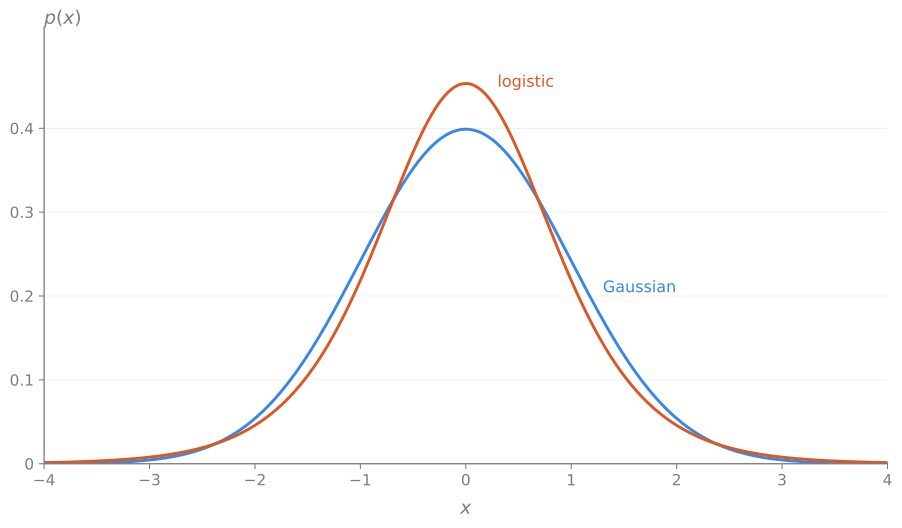
<p>However, note that this doesn’t uniquely determine the Gaussian. In fact, look how similar a Gaussian and a logistic distribution look:</p>

<figure>
  <center>
  <img src="/assets/blog/high-dimensional-space/the-n-dimensional-gaussian/gaussian-vs-logistic.svg" alt="A Gaussian vs a logistic distribution." />
  <figcaption><small><i>A Gaussian and a logistic distribution with similar scales. </i></small></figcaption>
  </center>
</figure>

<p>They are both smooth and symmetric, and aside from the logistic function’s heavier tail, there is little discernible detail between them visually. The Gaussian distribution arises from the following postulate.</p>

<div class="callout callout-note">

  <p><strong>The Gaussian postulate.</strong> For every dataset $\mathcal{D} = \{x_{1}, \cdots, x_{n}\}$, the most likely estimate of $\mu$ is the sample mean $\bar{x}$.</p>

</div>

<p>The rest of the derivation goes into a bit of detail, so I’ll wrap it up in a dropdown block.</p>

<details class="callout callout-why">
  <summary><b>Deriving the Gaussian distribution</b></summary>

  <p>By the postulate above, the maximum likelihood estimate (MLE) is</p>

\[\arg\max_{\mu}\prod_{i=1}^{n} \varphi(x_{i} - \mu) = \bar{x},\]

  <p>for every $n$ and every dataset $\mathcal{D}$.</p>

  <p>With the MLE our instinct is to convert it to log-likelihood, and set its derivative to zero.</p>

\[\begin{align}
\frac{d}{d\mu}\left[\sum_{i=1}^{n}\log\varphi(x_i-\mu)\right]
 &amp;= -\sum_{i=1}^{n}\frac{\varphi'(x_i - \mu)}{\varphi(x_i - \mu)} = 0.
\end{align}\]

  <p>Let $g(t) = \varphi’(t)/\varphi(t)$, so that we have</p>

\[\sum_{i=1}^{n}g(x_{i} - \mu) = 0.\]

  <p>Recall from the postulate that the maximum likelihood solution is $\mu = \bar{x}$, i.e.,</p>

\[\sum_{i=1}^{n}g(x_i - \bar{x}) = 0.\]

  <p>Let’s call the $r_i = x_i - \bar{x}$ the error residuals, which are actual quantities we have at our disposal; remember that we don’t know $\mu$, so we don’t have the errors $e_i = x_i - \mu$.</p>

  <p>We know that these residuals always sum up to zero:</p>

\[\sum_{i}^{n}r_{i} = \sum_{i}^{n}[x_i - \bar{x}] = \underbrace{(x_1 + \cdots + x_n)}_{n \cdot \bar{x}} - \, n\cdot \bar{x} = 0.\]

  <p>And from the postulate we know that their $g(\cdot)$ values also sum up to zero:</p>

\[\sum_{i}^{n}g(x_i - \bar{x}) = \sum_{i}^{n}g(r_i) = 0,\]

  <p>for every $n$ and every dataset $\mathcal{D}$. Given this, we can construct some datasets that give more information about the structure of $\varphi$.</p>

  <hr />

  <h3 id="case-1">Case 1</h3>

  <p>For $\mathcal{D} = \{x_1, x_2\}$ with $x_1 + x_2 = 0$, we have $\bar{x} = 0$ and</p>

\[\sum_{i=1}^{n}g(x_{i}) = g(x_1) + g(x_2) = 0.\]

  <p>This means that we have</p>

\[x_1 = -x_2 \qquad \Longrightarrow \qquad g(x_1) = -g(x_2), \tag{1} \label{eq:eq1}\]

  <p>which establishes that $g$ is an odd function:</p>

\[g(a) = -g(-a) \qquad \forall a \in \mathbb{R}.\]

  <hr />

  <h3 id="case-2">Case 2</h3>

  <p>For another $\mathcal{D} = \{x_1, x_2, x_3 \}$ with $x_1 + x_2 = -x_3$, we again have $\bar{x} = 0$ and</p>

\[\sum_{i=1}^{n}g(x_{i}) = g(x_1) + g(x_2) + g(x_3) = 0.\]

  <p>Moreover, from \eqref{eq:eq1} we have $g(x_3) = -g(-x_3)$. This gives</p>

\[\begin{align}
g(x_1) + g(x_2) &amp;= -g(x_3) \\
 &amp;= g(-x_3) \\
 &amp;= g(x_1 + x_2). \tag{2} \label{eq:eq2}
\end{align}\]

  <p>This is <a href="https://en.wikipedia.org/wiki/Cauchy%27s_functional_equation">Cauchy’s functional equation</a>.</p>

  <hr />

  <p>The only way to have the smooth, continuous $g$ satisfy both \eqref{eq:eq1} and \eqref{eq:eq2} is if $g(x)$ is a linear function, i.e.,</p>

\[g(x) = \frac{\varphi'(x)}{\varphi(x)} = \alpha\cdot x \qquad \text{for some } \alpha \in \mathbb{R},\]

  <p>and from this we derive that $\varphi(x)$ must be in the form of</p>

\[\begin{align}
\int \frac{\varphi'(x)}{\varphi(x)}\,dx &amp;= \int \alpha x\,dx \\
\log\varphi(x) &amp;= \frac{\alpha x^2}{2} + c \\
\varphi(x) &amp;= C e^{\alpha x^2 / 2} \qquad \text{for some } C &gt; 0.
\end{align}\]

  <p>We’ve recovered the general structure of $\varphi(x)$:</p>

\[\boxed{\varphi(x) = Ce^{\alpha x^2/2}}.\]

  <p>We now have to find what this $C$ is.</p>

  <hr />

  <p>Let us recall that $\varphi(x)$ corresponds to the density function of an actual probability distribution. In other words,
we need it to integrate to 1:</p>

\[\int_{-\infty}^{\infty} \varphi(x)\,dx = \int_{-\infty}^{\infty}Ce^{\alpha x^2/2}\,dx = 1.\]

  <p>This is only possible by having $\alpha &lt; 0$, so let’s use $\tau &gt; 0$ and describe $\varphi$ with $-\tau$ instead:</p>

\[\varphi(x) = C e^{-\tau x^2/2}.\]

  <p>Now we have</p>

\[C \int_{-\infty}^{\infty}e^{-(\tau/2)x^2}\,dx = 1.\]

  <p>Earlier during our derivation of the variance, we used the identity $\int_{-\infty}^{\infty}e^{-\beta x^2}\,dx = \sqrt{\pi/\beta}$. We can again use it here with $\beta = \tau/2$, which gives $\sqrt{2\pi/\tau}$. Then the normalizing constant $C$ is</p>

\[C \int_{-\infty}^{\infty}e^{(-\tau/2)x^2}\,dx = C \cdot \sqrt{\frac{2\pi}{\tau}} = 1 \qquad \Longrightarrow \qquad C = \sqrt{\frac{\tau}{2\pi}}.\]

  <p>Putting it all together, we have</p>

\[\varphi(x) = \sqrt{\frac{\tau}{2\pi}}e^{-\tau x^2/2}.\]

  <p>Using $p(x) = \varphi(x - \mu)$, we recover the Gaussian distribution density function $p(x)$ as</p>

\[p(x) = \varphi(x - \mu) = \sqrt{\frac{\tau}{2\pi}}e^{-\tau (x - \mu)^2 /2}.\]

  <p>This is a perfectly viable definition of the Gaussian distribution, using $\tau$ as the <strong>precision</strong> of the distribution. However, the standard formulation is by its variance $\sigma^2$, which we can obtain by the substitution $\tau = 1/\sigma^2$:</p>

\[\boxed{\mathcal{N}(x; \mu, \sigma^2) = \frac{1}{\sqrt{2\pi \sigma^2}} e^{-(x-\mu)^2/2\sigma^2}} \tag*{$\Box$}\]

  <p>The advantage of the $\sigma^2$-based parametrization is that we have the nice property of $\mathbb{V}[X] = \sigma^2$.</p>

</details>

<h2 id="the-multivariate-gaussian">The multivariate Gaussian</h2>

<p>We address the $n$-dimensional Gaussian more commonly as the <em>multivariate normal distribution</em>. It is the extension of the 1D case into multiple dimensions. The general form of the probability density function for the $n$-dimensional Gaussian is</p>

\[\mathcal{N}(\boldsymbol{\mu}, \mathbf{\Sigma}) = \frac{1}{(\sqrt{2\pi})^{n}}\cdot\frac{1}{\sqrt{\det\mathbf{\Sigma}}}\cdot \exp\left\{-\frac{1}{2}(\mathbf{x} - \boldsymbol{\mu})^{\top}\mathbf{\Sigma}^{-1}(\mathbf{x} - \boldsymbol{\mu})\right\},\]

<p>where $\boldsymbol{\mu} \in \mathbb{R}^{n}$ is the mean vector and $\mathbf{\Sigma}$ is a symmetric covariance matrix between the dimensions of the distribution. If we squint at it, it does resemble its univariate form.</p>

<p>The core property to remember is that each dimension in the distribution is itself a Gaussian distribution.</p>

<p>The multivariate Gaussian has two main categories, depending on the structure of its covariance matrix.</p>

<h3 id="isotropic-gaussians">Isotropic Gaussians</h3>

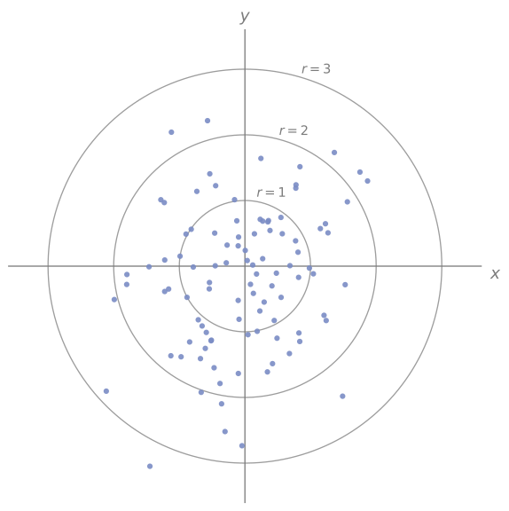
<p>An isotropic multivariate Gaussian is one where each dimension has the same variance $\sigma^2$, so $\mathbf{\Sigma} = \sigma^2\,I$:</p>

<figure>
  <center>
  <img src="/assets/blog/high-dimensional-space/the-n-dimensional-gaussian/gaussian-2d-contours-samples.svg" alt="An isotropic two-dimensional Gaussian distribution." />
  <figcaption><small><i>Samples from an isotropic two-dimensional Gaussian distribution with $\sigma^2 = 1.0$.</i></small></figcaption>
  </center>
</figure>

<p>They’re generally nice to work with.</p>

<p>We will later relate the $n$-dimensional unit ball to the $n$-dimensional isotropic Gaussian distribution. This intuitively makes a lot of sense because the unit ball and the isotropic Gaussian centered at the origin share a property called <em>rotational invariance</em>.</p>

<div class="callout callout-note">

  <p><strong>Rotational invariance.</strong> The isotropic Gaussian (with $\mu = 0$), the $n$-ball and the $(n-1)$-sphere are all rotational invariant. Rotation or choosing a new basis based on any random direction produces the same distribution, so they are all the same distribution in every direction.</p>

</div>

<h3 id="anisotropic-gaussians">Anisotropic Gaussians</h3>

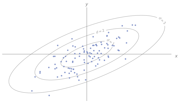
<p>A multivariate Gaussian can also be <em>anisotropic</em>, which means the individual dimensions have different variance and can correlate with each other:</p>

<figure>
  <center>
  <img src="/assets/blog/high-dimensional-space/the-n-dimensional-gaussian/gaussian-2d-contours-samples-correlated.svg" alt="An anisotropic two-dimensional Gaussian distribution." />
  <figcaption><small><i>An anisotropic 2D Gaussian with a canonical tilt.</i></small></figcaption>
  </center>
</figure>

<p>However, note that we can translate and rotate a Gaussian (i.e., choose new bases) and rescale each dimension’s variance to convert it into a standard normal distribution $\mathcal{N}(0, I_n)$. This is a common process known as <strong>whitening</strong>; all anisotropic Gaussians can be converted to isotropic Gaussians in this way.</p>

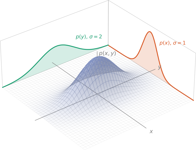
<p>The figure below shows that anisotropic Gaussians are still constructed out of 1D Gaussian distributions:</p>

<figure>
  <center>
  <img src="/assets/blog/high-dimensional-space/the-n-dimensional-gaussian/gaussian-2d-pdf-marginals-axis-aligned.svg" alt="Marginal view of a two-dimensional Gaussian distribution." />
  <figcaption><small><i>A two-dimensional Gaussian distribution decomposes into two one-dimensional marginal distributions.</i></small></figcaption>
  </center>
</figure>

<div class="callout callout-note">

  <p><strong>Takeaway</strong></p>

  <p>The marginal distribution of each dimension in the multivariate Gaussian is itself a Gaussian.</p>

</div>

<h2 id="scaling-the-gaussian-to-high-dimensions">Scaling the Gaussian to high dimensions</h2>

<p>Let’s look at the concentration of density of the Gaussian, as we did for the $n$-dimensional unit ball earlier.</p>

<h3 id="how-far-away-is-the-typical-point">How far away is the typical point?</h3>

<p>We have two similar ideas of the “mean” distance of a point. Our random variable of concern is $X \sim \mathcal{N}(\mu, \sigma^2)$.</p>

<h4 id="rms-distance">RMS distance</h4>

<p>The first one is the simple <strong>root-mean-square (RMS) distance</strong>, defined by</p>

\[d_{\mathrm{RMS}} = \sqrt{\mathbb{E}[(X - \mu)^2]}\]

<p>For the univariate Gaussian, we know that</p>

\[\sqrt{\mathbb{E}[(X - \mu)^2]} = \sqrt{\mathbb{V}[X]} = \sqrt{\sigma^2} = \sigma.\]

<p>This notion of distance generalizes to many other distributions as well.</p>

<h4 id="mean-absolute-distance">Mean absolute distance</h4>

<p>The second one is the mean absolute distance $\mathbb{E}\lvert X - \mu \rvert$.</p>

<p>For a one-dimensional Gaussian, it is equal to</p>

\[d_{\mathrm{abs}} = \mathbb{E}\lvert X - \mu \rvert = \sqrt{\frac{2}{\pi}}\sigma \approx 0.798 \sigma.\]

<details class="callout callout-why">
  <summary><b>Why?</b></summary>

  <p>We can make use of the symmetry of the distribution to simplify the required integral.</p>

\[\begin{align}
\mathbb{E}|x - \mu|
  &amp;= \int_{-\infty}^{\infty}\lvert x - \mu \rvert p(x)\,dx \\
  &amp;= 2\int_{\mu}^{\infty}(x-\mu)p(x)\,dx \\
  &amp;= 2\cdot\frac{1}{\sqrt{2\pi\sigma^2}}\int_{\mu}^{\infty} (x - \mu) e^{-(x - \mu)^2 / 2\sigma^2}\,dx \\
  &amp;= \frac{2}{\sqrt{2\pi\sigma^2}}\int_{0}^{\infty} u e^{-u^2/2\sigma^2}\,du \tag*{let $u = x - \mu$} \\
  &amp;= \frac{2}{\sqrt{2\pi\sigma^2}}\cdot \left[-\sigma^2 e^{-u^2/2\sigma^2}\right]_{0}^{\infty} \\
  &amp;= -\sqrt{\frac{2}{\pi}}\sigma [0 - 1] \\
  &amp;= \sqrt{\frac{2}{\pi}} \sigma.
\end{align}\]

</details>

<p>This result is more specific to the Gaussian, but it is literally what we mean by the distance of the point from the center.</p>

<h3 id="extension-to-the-multivariate-case">Extension to the multivariate case</h3>

<p>Recall that our intention is to look at the average distance of a sampled point from the $n$-dimensional Gaussian distribution. These two notions of distance don’t scale quite the same way <small>(…or do they?)</small></p>

<p>Let’s slightly make our work easier by sampling points from an isotropic multivariate Gaussian centered at the origin ($\boldsymbol{\mu} = 0$) with marginal variance $\sigma^2$ in all directions, so</p>

\[X \sim \mathcal{N}(0, \sigma^2 I).\]

<p>The corresponding radius is then $R = \lVert X  - \boldsymbol{\mu} \rVert = \lVert X \rVert$.</p>

<p><strong>The RMS distance.</strong> This one behaves quite nicely, given that</p>

\[\mathbb{E}[R^2] = \sum_{i=1}^{n}\mathbb{E}[(X_{i})^2] = n\sigma^2,\]

<p>meaning that we have</p>

\[d_{\mathrm{RMS}} = \sqrt{\mathbb{E}[R^2]} = \sigma\sqrt{n}.\]

<p>This indicates that distance of the typical point from the Gaussian, based on $d_{\mathrm{RMS}}$, is around an $(n-1)$-sphere of radius $\sigma\sqrt{n}$. Before reaching a conclusion, let’s check if this also applies to the other distance as well.</p>

<hr />

<p><strong>The actual expected distance from the center.</strong> Recall that we showed that the mean absolute distance for the 1D case is</p>

\[d_{\mathrm{abs}} = \mathbb{E}\lvert x - \mu \rvert = \sqrt{\frac{2}{\pi}}\sigma \approx 0.798 \sigma.\]

<p>Scaling this to $n$ dimensions is not as straightforward as it might first seem.</p>

<p>The quantity we’re after here is the actual distance, obtained by</p>

\[\mathbb{E}[R] = \mathbb{E}\lVert X \rVert = \mathbb{E}\sqrt{\sum_{i=1}^{n}{X_{i}^2}}.\]

<p>The derivation of this is in the <a href="#appendix">appendix</a>, but we see that this value is equal to</p>

\[\boxed{\mathbb{E}[R] = \sigma\sqrt{2}\,\frac{\Gamma\!\left(\frac{n+1}{2}\right)}{\Gamma\!\left(\frac{n}{2}\right)}}\]

<p>with $\Gamma(z)$ being Euler’s Gamma function that we saw before in the <a href="/blog/2026/09/20/the-volume-of-the-n-ball/">volume of the $n$-ball</a>. As a quick check, $n=1$ gives us $\sqrt{2}\left[\Gamma(1)/\Gamma(1/2)\right] = \sqrt{2/\pi}$, which is what we found for the 1D case previously with $\sigma^2 = 1$.</p>

<p>As $n \to \infty$, we see that this expectation also behaves like</p>

\[\mathbb{E}[R] \approx \sigma\sqrt{n}.\]

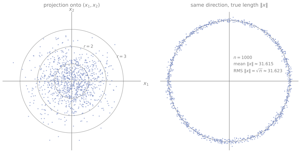
<p>So the two distances kinda converge to the same “shell”. It’s best to verify this visually as well:</p>

<figure class="post-figure">
  <img src="/assets/blog/high-dimensional-space/the-n-dimensional-gaussian/gaussian-high-dim-projection-vs-norm.svg" alt="2D projection of a 1000-dimensional Gaussian, and their true lengths." />
  <figcaption>Projection of a $1000$-dimensional Gaussian onto the XY plane, and plotting its norm.</figcaption>
</figure>

<p><strong>Left figure:</strong> Since all of the individual coordinates are independent from each other for a Gaussian, a 2D projection of an $n$-dimensional Gaussian looks, well, exactly like a 2D Gaussian.</p>

<p><strong>Right figure:</strong> What we’ve uncovered is that plotting their distances to the center should give us something like a “thin shell”, which is reminiscent of a sphere.</p>

<hr />

<p>What’s more, the variance of this radius is bounded by $\sigma^2$ (again, shown in the <a href="#appendix">appendix</a>): we have</p>

\[\sigma\sqrt{n-1} \le \mathbb{E}[R] \le \sigma\sqrt n,\]

<p>which can be used to bound the variance</p>

\[\mathbb{V}[R] = \mathbb{E}[R^2] - (\mathbb{E}[R])^2 \leq n \sigma^2 - (n-1) \sigma^2 = \sigma^2,\]

<p>which indicates that the variance of the thin shell is actually bounded <strong>independent of the dimension</strong> $n$.</p>

<p>In fact, we know that the radius of the shell grows like $\sigma\sqrt{n}$, but its spread $\sqrt{\mathbb{V}[R]}$ doesn’t grow at all. Comparing the two we have</p>

\[\frac{\sqrt{\mathbb{V}[R]}}{\mathbb{E}[R]} \le \frac{\sigma}{\sigma\sqrt{n-1}} = \frac{1}{\sqrt{n-1}},\]

<p>so the shell’s thickness relative to its radius shrinks like $1/\sqrt{n}$.</p>

<div class="callout callout-note">

  <p><strong>The “thin shell”</strong></p>

  <p>The typical point sampled from a Gaussian sits on a thin shell at radius $\sigma\sqrt{n}$. This shell has a fixed absolute thickness, and becomes ever thinner relative to its size as $n$ increases.</p>

</div>

<h2 id="comparing-the-ball-the-sphere-and-the-gaussian">Comparing the ball, the sphere, and the Gaussian</h2>

<p>In <a href="/blog/2026/09/20/the-volume-of-the-n-ball/">the volume of the n-ball</a>, we saw how we can uniformly sample from the unit sphere by sampling a vector $\mathbf{v}$ from a multivariate Gaussian and normalizing it with $\mathbf{v} \leftarrow \mathbf{v} / \lVert \mathbf{v} \rVert$ exploiting rotational symmetry. We could also sample from the unit ball as well by scaling the sphere result with $U^{1/n}$.</p>

<p>Let’s uncover more about these three, from the other direction this time.</p>

<hr />

<p>One interesting comparison opportunity arises from comparing the marginal distributions for each of these three objects.</p>

<p>From the <a href="/blog/2026/09/20/the-volume-of-the-n-ball/">volume post</a>, we know that the unit ball $B_{n}$ has a marginal probability of</p>

\[p(t) \propto (1-t^2)^{(n-1)/2},\]

<p>and from the earlier <a href="/blog/2026/09/25/the-surface-of-the-n-ball/">surface post</a> we know the unit sphere $S_{n-1}$ has a marginal probability of</p>

\[p(t) \propto (1-t^2)^{(n-3)/2}.\]

<p>Finally, we know (from this post) that the Gaussian has independent coordinates with marginal probabilities of</p>

\[p(t) = \mathcal{N}(t; 0, \sigma^2).\]

<p>Let’s scale it with $\sigma^2 = \frac{1}{n}$, so that its points form a thin shell around $R = \sigma\sqrt{n} = 1$, just like the boundaries of the ball and sphere.</p>

<p>Here’s how the marginal distributions of the unit $n$-ball and the $(n-1)$-sphere change with increasing dimensionality, compared to a scaled Gaussian with $\sigma^2 = \tfrac1n$:</p>

<table class="table-centered">
  <thead>
    <tr>
      <th>$n$</th>
      <th>$n$-ball</th>
      <th>$(n-1)$-sphere</th>
      <th>Gaussian</th>
    </tr>
  </thead>
  <tbody>
    <tr>
      <td>1</td>
      <td>uniform on $[-1,1]$</td>
      <td>two points: $-1, +1$</td>
      <td>$\mathcal{N}(0, \tfrac1n)$</td>
    </tr>
    <tr>
      <td>2</td>
      <td>semicircle $\sqrt{1-t^2}$</td>
      <td>arcsine, $\frac{1}{\sqrt{1-t^2}}$</td>
      <td>$\mathcal{N}(0, \tfrac1n)$</td>
    </tr>
    <tr>
      <td>3</td>
      <td>parabola $1-t^2$</td>
      <td>uniform</td>
      <td>$\mathcal{N}(0, \tfrac1n)$</td>
    </tr>
    <tr>
      <td>large</td>
      <td>$\approx \mathcal{N}(0, \tfrac1n)$</td>
      <td>$\approx \mathcal{N}(0, \tfrac1n)$</td>
      <td>$\mathcal{N}(0, \tfrac1n)$</td>
    </tr>
  </tbody>
</table>

<p>The uniformly distributed cases of $n=1$ for the ball and $n=3$ for the sphere are quite interesting (the 2-sphere’s uniform distribution is Archimedes’ remarkable <a href="https://mathworld.wolfram.com/ArchimedesHat-BoxTheorem.html">hat-box theorem</a>!), however, we see that in the asymptotic case these three all blend into each other.</p>

<p>Of course, the marginal distributions are interesting, however the joint distribution is what uniquely determines the particular distribution. The unit cube and the $2$-sphere both have uniform marginals for $x$, $y$, and $z$, however the sphere’s joint distribution is also constrained by the requirement of $x^2 + y^2 + z^2 = R^2$ for some $R \geq 0$.</p>

<p>This leads us to the unique property of Gaussians, as stated by <a href="https://en.wikipedia.org/wiki/Maxwell%27s_theorem">Herschel-Maxwell’s theorem</a>:</p>

<div class="callout callout-note">

  <p><strong>Herschel-Maxwell’s theorem</strong></p>

  <p>The centered isotropic Gaussian is the only distribution that is both rotationally symmetric and has independent coordinates.
The ball and sphere have the symmetry without independence, and an axis-aligned anisotropic Gaussian has independence but not symmetry. It is only the centered isotropic Gaussian with $n \geq 2$ that has both.</p>

</div>

<p>Fun fact! This property was derived from Herschel’s 1850 work on measurements of astronomical star positions, and extended with Maxwell’s 1860 analysis of gas molecule velocities.</p>

<hr />

<p>The important takeaway of the story is that with increasingly larger $n$ (and appropriate scaling), the line between a ball, a sphere, and a (scaled) Gaussian seems to blur into the same thing:</p>

<ul>
  <li>
    <p>We saw previously that the volume of the $n$-ball is increasingly concentrated near its boundary, which is the $(n-1)$-sphere.</p>
  </li>
  <li>
    <p>We see that the typical point of a Gaussian concentrates again on a thin shell around $\sigma\sqrt{n}$, which resembles a sphere of radius $\sigma\sqrt{n}$.</p>
  </li>
</ul>

<div class="callout callout-note">

  <p>The main difference of the Gaussian, most prominent for lower $n$, is that it is not bounded to a specific radius (unlike the ball and the sphere), and that the coordinates are independent of each other.</p>

  <p>With larger $n$, the differences between the three decrease as a consequence of high dimensional geometry.</p>

</div>

<hr />

<h2 id="closing-remarks">Closing remarks</h2>

<p>There is obviously so much more about Gaussians in high dimensional space, but I think this is a good point to finish the post in terms of length. I might revisit this topic again soon though.</p>

<p>I think the next post will be on distances and angles. It will probably start off from the very famous property of <strong>near-orthogonality</strong> of random vectors, and will continue from our Gaussian discussion:</p>

<div class="callout callout-note">

  <p>In high dimensional space, two random vectors sampled from a Gaussian distribution are nearly orthogonal with high probability.</p>

</div>

<hr />

<h2 id="appendix">Appendix</h2>

<h3 id="deriving-mathbber">Deriving $\mathbb{E}[R]$</h3>

<p>Throughout this section we have $X \sim \mathcal{N}(0, \sigma^2 I_n)$ and $R = \lVert X \rVert$. Claude was a huge help in the main idea and the heavier math parts.</p>

<p>The idea is to find the distribution of $R$, and then compute the moments of $R$. $\mathbb{E}[R^m]$ is called the $m$-th (raw) moment of $R$, and we’ll use the first and second raw moments to find $\mathbb{E}[R]$ and $\mathbb{V}[R]$.</p>

<p>We’ll proceed in a series of steps.</p>

<h4 id="step-1-the-distribution-of-the-radius-via-the-onion-method">Step 1: the distribution of the radius via the onion method</h4>

<p>How is $R$ distributed? Since the Gaussian is unbounded, technically any radius is possible. We’re going to use the same onion method from the surface post.</p>

<hr />

<p>The density of the isotropic Gaussian only depends on $\mathbf{x}$ through its length $r = \lVert \mathbf{x} \rVert$:</p>

\[p(\mathbf{x}) = \frac{1}{(2\pi\sigma^2)^{n/2}}\,e^{-\lVert \mathbf{x} \rVert^2/2\sigma^2}.\]

<p>So the density is constant on every sphere centered at the origin, and we can slice $\mathbb{R}^n$ into onion layers, just like in the <a href="/blog/2026/09/25/the-surface-of-the-n-ball/">surface post</a>. The probability of landing in the thin shell between $r$ and $(r + dr)$ is the density on that shell multiplied by the shell’s volume, $S_{n-1}(r)\,dr$:</p>

\[P(r \le R \le r + dr) \approx p(\mathbf{x})\Big|_{\lVert \mathbf{x} \rVert = r} \cdot S_{n-1}(r)\,dr.\]

<p>Using $S_{n-1}(r) = \frac{2\pi^{n/2}}{\Gamma(n/2)}r^{n-1}$, the density of $R$ is</p>

\[\begin{align}
p_R(r) &amp;= \frac{2\pi^{n/2}}{\Gamma(n/2)}\,r^{n-1}\cdot\frac{1}{(2\pi\sigma^2)^{n/2}}\,e^{-r^2/2\sigma^2} \\
 &amp;= \frac{2}{(2\sigma^2)^{n/2}\,\Gamma(n/2)}\,r^{n-1}\,e^{-r^2/2\sigma^2}, \qquad r \ge 0. \tag{A1} \label{eq:radial}
\end{align}\]

<p>Conceptually, the two factors pull in opposite directions: $r^{n-1}$ (the sphere getting bigger) pushes the mass outwards, while $e^{-r^2/2\sigma^2}$ (the Gaussian) pulls it back in. The thin shell is where these two balance out.</p>

<div class="callout callout-note">

  <p>$p_R$ is known as the (scaled) <a href="https://en.wikipedia.org/wiki/Chi_distribution">chi distribution</a> with $n$ degrees of freedom; its square $R^2/\sigma^2$ is the more familiar chi-squared distribution.</p>

</div>

<h4 id="step-2-one-integral-for-every-moment">Step 2: one integral for every moment</h4>

<p>Every moment $\mathbb{E}[R^m]$ needs an integral of the form $\int_0^\infty r^k e^{-r^2/2\sigma^2}\,dr$, so let’s do it once. Recall that the Gamma function is defined by</p>

\[\Gamma(z) = \int_0^\infty t^{z-1}e^{-t}\,dt, \qquad z &gt; 0.\]

<p>We have</p>

\[\int_0^\infty r^k e^{-r^2/2\sigma^2}\,dr = \frac{1}{2}(2\sigma^2)^{(k+1)/2}\,\Gamma\!\left(\frac{k+1}{2}\right). \tag{A2} \label{eq:gammaint}\]

<details class="callout callout-why">
  <summary><b>Why is the integral a Gamma function?</b></summary>

  <p>Substitute $t = r^2/2\sigma^2$, so that</p>

\[r = (2\sigma^2 t)^{1/2}, \qquad dr = \frac{1}{2}(2\sigma^2)^{1/2}\,t^{-1/2}\,dt.\]

  <p>Then</p>

\[\begin{align}
\int_0^\infty r^k e^{-r^2/2\sigma^2}\,dr
 &amp;= \int_0^\infty (2\sigma^2 t)^{k/2}\,e^{-t}\cdot\frac{1}{2}(2\sigma^2)^{1/2}\,t^{-1/2}\,dt \\
 &amp;= \frac{1}{2}(2\sigma^2)^{(k+1)/2}\int_0^\infty t^{(k-1)/2}e^{-t}\,dt \\
 &amp;= \frac{1}{2}(2\sigma^2)^{(k+1)/2}\,\Gamma\!\left(\tfrac{k+1}{2}\right).
\end{align}\]

</details>

<p>Now the $m$-th moment of $R$ is \eqref{eq:radial} multiplied by $r^m$, i.e. \eqref{eq:gammaint} with $k = n - 1 + m$:</p>

\[\begin{align}
\mathbb{E}[R^m] &amp;= \frac{2}{(2\sigma^2)^{n/2}\,\Gamma(n/2)}\int_0^\infty r^{n-1+m}e^{-r^2/2\sigma^2}\,dr \\
 &amp;= \frac{2}{(2\sigma^2)^{n/2}\,\Gamma(n/2)}\cdot\frac{1}{2}(2\sigma^2)^{(n+m)/2}\,\Gamma\!\left(\frac{n+m}{2}\right) \\
 &amp;= (2\sigma^2)^{m/2}\,\frac{\Gamma\!\left(\frac{n+m}{2}\right)}{\Gamma\!\left(\frac{n}{2}\right)}. \tag{A3} \label{eq:moments}
\end{align}\]

<p>Let’s do a sanity check on \eqref{eq:moments} with two values before using it:</p>

<ul>
  <li>$m = 0$ gives $\mathbb{E}[1] = \Gamma(n/2)/\Gamma(n/2) = 1$, so $p_R$ integrates to $1$ as a density should.</li>
  <li>$m = 2$ gives $2\sigma^2\cdot\Gamma(\frac{n}{2} + 1)/\Gamma(\frac{n}{2}) = 2\sigma^2\cdot\frac{n}{2} = n\sigma^2$ using $\Gamma(z+1) = z\Gamma(z)$, which matches the RMS result $\mathbb{E}[R^2] = n\sigma^2$ from the main text.</li>
</ul>

<h4 id="step-3-the-expected-radius">Step 3: the expected radius</h4>

<p>With $m = 1$ we get our result:</p>

\[\boxed{\mathbb{E}[R] = \sigma\sqrt{2}\,\frac{\Gamma\!\left(\frac{n+1}{2}\right)}{\Gamma\!\left(\frac{n}{2}\right)}}. \tag*{$\Box$}\]

<p>For $n = 1$, $\Gamma(1) = 1$ and $\Gamma(\frac{1}{2}) = \sqrt{\pi}$ give $\sqrt{2/\pi}\,\sigma$, the mean absolute distance from the 1D case.</p>

<h3 id="bounding-mathbber-and-mathbbvr">Bounding $\mathbb{E}[R]$ and $\mathbb{V}[R]$</h3>

<p>We now show that</p>

\[\sigma\sqrt{n-1} \;\le\; \mathbb{E}[R] \;\le\; \sigma\sqrt{n}.\]

<p>In the appendix of the <a href="/blog/2026/09/25/the-surface-of-the-n-ball/">surface post</a>, we defined</p>

\[g(x) = \frac{\Gamma(x+1)}{\Gamma(x+\frac{1}{2})}\]

<p>and showed with the squeeze theorem that for $x &gt; 0$,</p>

\[\sqrt{x} \le g(x) \le \sqrt{x + \tfrac{1}{2}}.\]

<p>The Gamma ratio in $\mathbb{E}[R]$ is exactly $g$ in disguise: setting $x = \frac{n-1}{2}$ gives $x + 1 = \frac{n+1}{2}$ and $x + \frac{1}{2} = \frac{n}{2}$, so</p>

\[\mathbb{E}[R] = \sigma\sqrt{2}\cdot g\!\left(\tfrac{n-1}{2}\right).\]

<p>Applying the bounds for $n \ge 2$:</p>

\[\sigma\sqrt{2}\cdot\sqrt{\frac{n-1}{2}} \;\le\; \mathbb{E}[R] \;\le\; \sigma\sqrt{2}\cdot\sqrt{\frac{n}{2}}
\qquad\Longrightarrow\qquad
\sigma\sqrt{n-1} \;\le\; \mathbb{E}[R] \;\le\; \sigma\sqrt{n}.\]

<p>The case $n = 1$ can be checked directly, since $0 \le \sqrt{2/\pi}\,\sigma \approx 0.798\,\sigma \le \sigma$. $\Box$</p>

<div class="callout callout-note">

  <p>The upper bound also follows in one line from Jensen’s inequality, since the square root is concave:</p>

\[\mathbb{E}[R] = \mathbb{E}\big[\sqrt{R^2}\big] \le \sqrt{\mathbb{E}[R^2]} = \sigma\sqrt{n}.\]

</div>

<hr />

<p>We can now follow this up with the variance bound. Using $\mathbb{E}[R^2] = n\sigma^2$ and the lower bound on $\mathbb{E}[R]$,</p>

\[\mathbb{V}[R] = \mathbb{E}[R^2] - (\mathbb{E}[R])^2 \le n\sigma^2 - (n-1)\sigma^2 = \sigma^2. \tag*{$\Box$}\]]]></content><author><name>Çağrı Eser</name></author><summary type="html"><![CDATA[I talk about the multivariate normal distribution's properties in high-dimensional space.]]></summary><media:thumbnail xmlns:media="http://search.yahoo.com/mrss/" url="https://cagrislist.org/assets/blog/thumbs/the-n-dimensional-gaussian.png" /><media:content medium="image" url="https://cagrislist.org/assets/blog/thumbs/the-n-dimensional-gaussian.png" xmlns:media="http://search.yahoo.com/mrss/" /></entry><entry><title type="html">The surface of the n-ball</title><link href="https://cagrislist.org/blog/2026/09/25/the-surface-of-the-n-ball/" rel="alternate" type="text/html" title="The surface of the n-ball" /><published>2026-09-25T00:00:00+00:00</published><updated>2026-09-25T00:00:00+00:00</updated><id>https://cagrislist.org/blog/2026/09/25/the-surface-of-the-n-ball</id><content type="html" xml:base="https://cagrislist.org/blog/2026/09/25/the-surface-of-the-n-ball/"><![CDATA[<p class="callout"><small> This is the third entry in the
<a href="/blog/2026/09/16/a-leap-into-high-dimensional-space/">high-dimensional space blog series</a>.
</small></p>

<p>Let’s talk about another simple way of calculating the volume of the $n$-ball, with a method that on paper seems more intuitive than the cross-section approach.</p>

<p>I had planned this one to have less math than the previous post, but it turned out to require even more! It’s nice that the “mathy” blocks can be toggled on/off with the <strong>“Why?”</strong> blocks.</p>

<h2 id="the-onion-method">The onion method</h2>

<p>Recall that in <a href="/blog/2026/09/16/the-volume-of-the-four-ball/">the volume of the 4-ball</a>, we showed that the 2D disk can be thought of as a vertical stack of horizontal disks, which were actually $1$-balls of varying radii:</p>

<figure>
  <center>
  <img src="/assets/blog/high-dimensional-space/disk-2d-slices.svg" alt="2D disk as a stack of 1D intervals." />
  <figcaption><small><i>The disk is a vertical stack of $1$-balls.</i></small></figcaption>
  </center>
</figure>

<p>If we’re going to be slicing up the unit ball, there is a much more intuitive way of doing so: radially outwards, like an onion.</p>

<figure>
  <center>
  <img src="/assets/blog/high-dimensional-space/the-surface-of-the-n-ball/disk-concentric-circles.svg" alt="2D disk as a stack of 1-spheres." />
  <figcaption><small><i>The disk is a radial stack of circles.</i></small></figcaption>
  </center>
</figure>

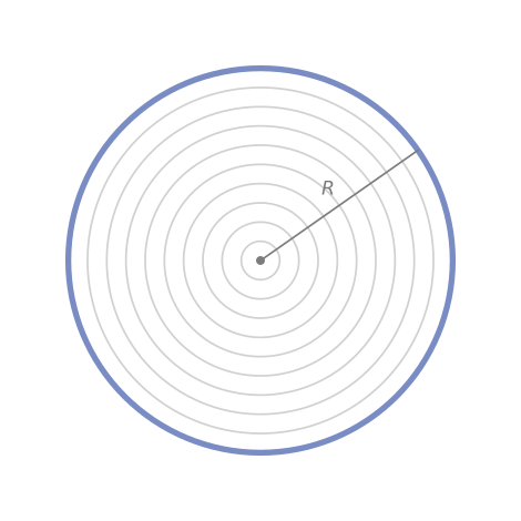
<p>Inside a disk of radius $R$, each one of these circles has a circumference of $2\pi r$ with varying $r \in [0, R]$. The integral for adding all of these circle circumferences gives us the volume:</p>

\[V_{2}(R) = \int_{0}^{R} 2\pi r\,dr = \pi R^{2}.\]

<p>That was pretty easy, wasn’t it?</p>

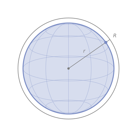
<p>This also works in the three-dimensional case as well. We know that the surface of the ball of radius $R$ has a surface area of $4\pi R^{2}$, and the $3$-ball can be thought of as a similar 3D onion with infinite layers.</p>

<figure>
  <center>
  <img src="/assets/blog/high-dimensional-space/the-surface-of-the-n-ball/ball-concentric-spheres.svg" alt="The 3-ball as a stack of spheres." />
  <figcaption><small><i>The $3$-ball is a radial stack of $2$-spheres.</i></small></figcaption>
  </center>
</figure>

<p>Again, we find that the integral here gives us the volume of the $3$-ball.</p>

\[V_{3}(R) = \int_{0}^{R} 4\pi r^2 \,dr = \frac{4}{3}\pi R^3.\]

<div class="callout">

  <h3 id="a-note-on-terminology">A note on terminology</h3>

  <p>Do note by definition that the $n$-sphere bounds the $(n+1)$-ball. Some examples:</p>

  <ul>
    <li>The $0$-sphere is just two points $\left\{ x - R, x + R \right\}$ that bound the $1$-ball $B(x; R)$ that is centered on $x$ with radius $R$.</li>
    <li>The $1$-sphere is our good friend, the circle.</li>
    <li>The $2$-sphere is the hollow shell of the $3$-ball, like the glass part of a snowglobe.</li>
  </ul>

</div>

<h3 id="the-n-dimensional-case">The n-dimensional case</h3>

<p>So why didn’t we use this for volume of the $n$-ball, as it looks easier to calculate? It’s because we didn’t know the surface area of the $n$-ball, of course!</p>

<p>We actually go the other way around: the surface area $S_{n-1}(R)$ for the $n$-ball is the volume of the $(n-1)$-sphere, and is equal to the rate of change of the volume of the $n$-ball with respect to the radius:</p>

\[\begin{align}
S_{n-1}(R) &amp;= \frac{d}{dR}V_{n}(R) \\
           &amp;= \boxed{\frac{2\pi^{n/2}}{\Gamma(n/2)}R^{n-1}}. \label{eq:eq1} \tag{1}
\end{align}\]

<p>And by our onion construction, we can express the volume of the $n$-ball using the volume of the $(n-1)$-sphere as</p>

\[\boxed{V_{n}(R) = \int_{0}^{R} S_{n-1}(r)\,dr}. \label{eq:eq2} \tag{2}\]

<details open="" class="callout">
  <summary><b>Why?</b></summary>

  <p>Suppose we are looking at the difference between $V_{n}(R)$ and $V_{n}(R + h)$ for some $h &gt; 0$. Intuitively, this is the volume of the shell between two nested $n$-balls, and as $h \to 0$ this approximates the boundary of the ball of radius $R$, which is the sphere of radius $R$ multiplied by a height of $h$.</p>

\[\begin{align}
V_n(R+h) - V_n(R) &amp;\approx S_{n-1}(R)\cdot h \\
\quad\Longrightarrow\quad
S_{n-1}(R) &amp;= \lim_{h\to 0}\frac{V_n(R+h) - V_n(R)}{h} = V_n'(R).
\end{align}\]

  <p>Therefore we have</p>

\[\begin{align}
S_{n-1}(R) := V'_{n}(R) &amp;= \frac{d}{dR} \left[\frac{\pi^{n/2}}{\Gamma(n/2 + 1)}R^{n}\right] \\
  &amp;= \frac{\pi^{n/2}}{\Gamma(n/2 + 1)}\cdot\frac{d}{dR}[R^n] \\
  &amp;= \frac{\pi^{n/2}}{\Gamma(n/2 + 1)}\cdot n \cdot R^{n-1} \\
  &amp;= \frac{\pi^{n/2}}{\frac{n}{2}\Gamma(n/2)}\cdot n \cdot R^{n-1} \\
  &amp;= \frac{2\pi^{n/2}}{\Gamma(n/2)}R^{n-1}.
\end{align}\]

  <p>which recovers \eqref{eq:eq1}. It then follows from $S_{n-1}(R) = \frac{d}{dR}V_{n}(R)$ that</p>

\[\int_{0}^{R} S_{n-1}(r)\,dr = V_{n}(R) - V_{n}(0) = V_{n}(R),\]

  <p>which gives us \eqref{eq:eq2}.</p>

</details>

<h2 id="does-the-onion-method-always-work">Does the onion method always work?</h2>

<p>In the volume post, there was one nice property that we didn’t touch upon: Fubini’s theorem and the cross-section idea work not just for Euclidean distance, but for other norms as well.</p>

<p>An $\ell_{p}$ norm for a vector $\mathbf{u} \in \mathbb{R}^n$ is a measure for the length of a vector $\mathbf{u}$, defined as:</p>

\[\ell_{p}(\mathbf{u}) = \lVert \mathbf{u} \rVert_{p} = \left(\lvert u_{1}\rvert^{p} + \lvert u_{2}\rvert^p + \cdots + \lvert u_{n}\rvert^p\right) ^{1/p}.\]

<p>For $p=2$, this is our good old Euclidean distance, for example for $\mathbf{u} \in \mathbb{R}^3$ with $\mathbf{u} = (x, y, z)$:</p>

\[\ell_{2}(\mathbf{u}) = \lVert \mathbf{u} \rVert_{2} = \sqrt{x^2 + y^2 + z^2}.\]

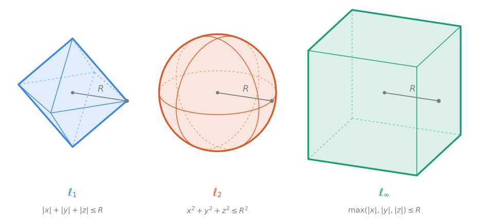
<p>The shapes below are all $3$-balls, just with different norms.</p>
<figure>
  <center>
  <img src="/assets/blog/high-dimensional-space/the-surface-of-the-n-ball/lp-balls-3d.svg" alt="3-balls of all shapes and sizes." />
  <figcaption><small><i>The 3-ball equipped with other norms.</i></small></figcaption>
  </center>
</figure>

<p>The green ball (cube) uses the max norm. The max-norm is the resulting norm we have as $p \to \infty$. It is defined as</p>

\[\ell_{\infty}(\mathbf{u}) = \lVert \mathbf{u} \rVert_{\infty} = \max\left\{|u_{1}|, |u_{2}|, \cdots ,|u_{n}| \right\}.\]

<div class="callout">

  <h4 id="practical-insight-into-the-ellp-norms">Practical insight into the $\ell_p$ norms</h4>

  <ul>
    <li>
      <p>In 2D, $\ell_{1}$ norm is the minimum distance you would need to go to reach a target point if you could only move horizontally or vertically.</p>
    </li>
    <li>
      <p>The $\ell_{\infty}$ norm is like the king in chess: moving diagonally costs the same as moving horizontally or vertically.</p>
    </li>
    <li>
      <p>$\ell_{2}$ norm is our “default” distance based on the hypotenuse of the triangle.</p>
    </li>
  </ul>

</div>

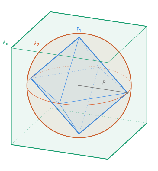
<p>What’s also cool is that they all encapsulate each other with increasing $p$:</p>

<figure>
  <center>
  <img src="/assets/blog/high-dimensional-space/the-surface-of-the-n-ball/lp-balls-3d-overlay.svg" alt="Nested 3-balls of different norms." />
  <figcaption><small><i>The $3$-balls all fit inside one another.</i></small></figcaption>
  </center>
</figure>

<p>We’re going to talk about norms and distances in greater detail in a later post.</p>

<h3 id="so-why-talk-about-the-norm-now">So why talk about the norm now?</h3>

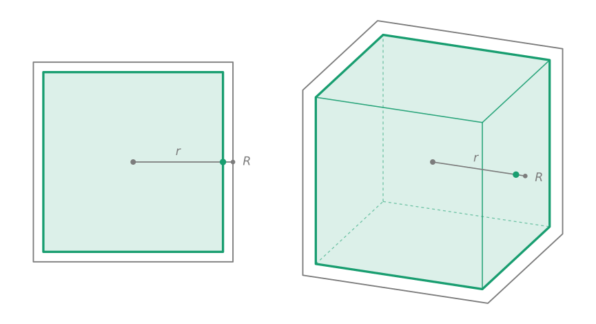
<p>Our onion approach is a special case of the $\ell_2$ (Euclidean) norm. Interestingly enough, it also holds for the $\ell_{\infty}$ norm as well.</p>

<figure>
  <center>
  <img src="/assets/blog/high-dimensional-space/the-surface-of-the-n-ball/square-cube-concentric-shells.svg" alt="The onion method with the max norm." />
  <figcaption><small><i>The onion method with the $\ell_{\infty}$ norm.</i></small></figcaption>
  </center>
</figure>

<ul>
  <li>With $\ell_{\infty}$, the “$1$-sphere” of radius $r$ gives us a square of $4$ edges of length $2r$. Integrating this gives us</li>
</ul>

\[V_{2}(R) = \int_{0}^{R} 4\cdot2r\,dr = 4R^2,\]

<p>which is the volume of the “$2$-ball” here, the square of edge length $2R$.</p>

<ul>
  <li>In 3D this again holds: a max norm $2$-sphere of radius $r$ has $6$ faces of surface area $2r \times 2r = 4r^2$, and integrating gives us</li>
</ul>

\[V_{3}(R) = \int_{0}^{R} 6 \cdot 4r^{2}\,dr = 8 R^3,\]

<p>which is again the volume of the $3$-ball with max norm, in other words, a cube with edge length $2R$ with volume $(2R)^3 = 8R^3$.</p>

<hr />

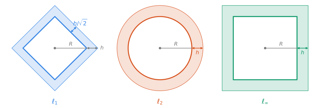
<p>For other norms though, we have the issue of slantedness. It’s most intuitively observed in the figure below for the disk with various $\ell_{p}$ norms.</p>

<figure>
  <center>
  <img src="/assets/blog/high-dimensional-space/the-surface-of-the-n-ball/lp-disks-shell-thickness.svg" alt="The thin shell formed by increasing radius R by h." />
  <figcaption><small><i>The shell obtained from increasing $R$ by $h$.</i></small></figcaption>
  </center>
</figure>

<p>In our argument above we said that for sufficiently small $h &gt; 0$ the difference between the volumes of the $n$-ball of radius $(R+h)$ and $R$ can be approximated by $S_{n-1}(R) \cdot h$.</p>

<p>Uniquely for $\ell_{2}$ and $\ell_{\infty}$, we see that increasing the radius $R$ by some $h$ directly pushes the outer shell away by $h$, whereas there is a slant factor for all other $\ell_{p}$ norms (for example, $\ell_{1}$ has $\frac{h}{\sqrt{2}}$ instead). That means we can’t use the $S_{n-1}(R) \cdot h$ volume approximation for the other norms.</p>

<div class="callout">

  <p>To summarize: \eqref{eq:eq2} holds for all dimensions, but only for $\ell_2$ and $\ell_{\infty}$ among all of the $\ell_p$ norms.</p>

</div>

<h2 id="the-rollercoaster-of-the-volume-of-the-n-1-sphere">The rollercoaster of the volume of the $(n-1)$-sphere</h2>

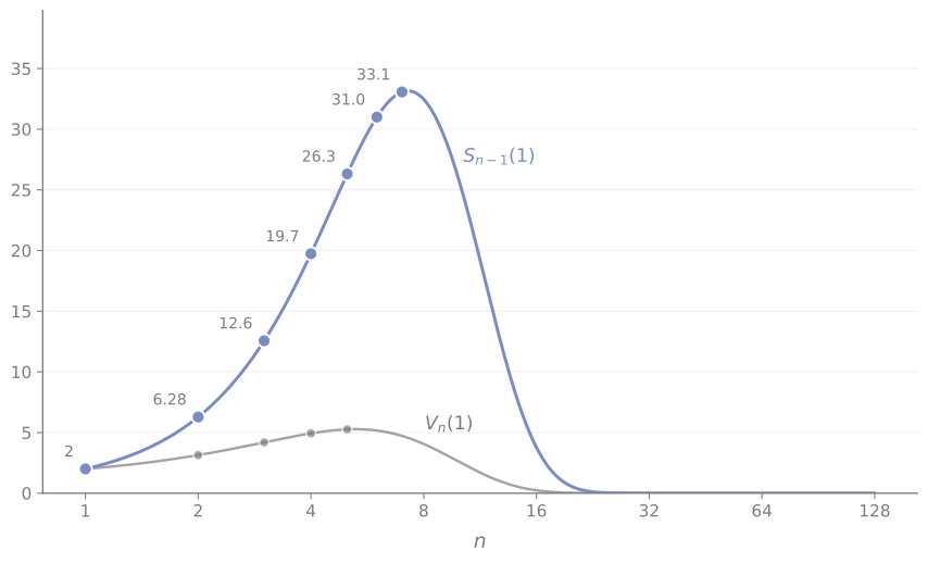
<p>Given that Eq. \eqref{eq:eq1} looks awfully similar to the <a href="/blog/2026/09/20/the-volume-of-the-n-ball/">$n$-ball volume formula</a>, we might expect this next property: the volume $S_{n-1}(R)$ of the $(n-1)$-sphere with radius $R$ also increases for a bit before superexponentially plummeting to zero.</p>

<figure>
  <center>
  <img src="/assets/blog/high-dimensional-space/the-surface-of-the-n-ball/surface-and-volume-vs-dimension-log.svg" alt="Unit sphere and volume against dimension." />
  <figcaption><small><i>Plotting the hypervolume of the unit sphere and ball against $n$.</i></small></figcaption>
  </center>
</figure>

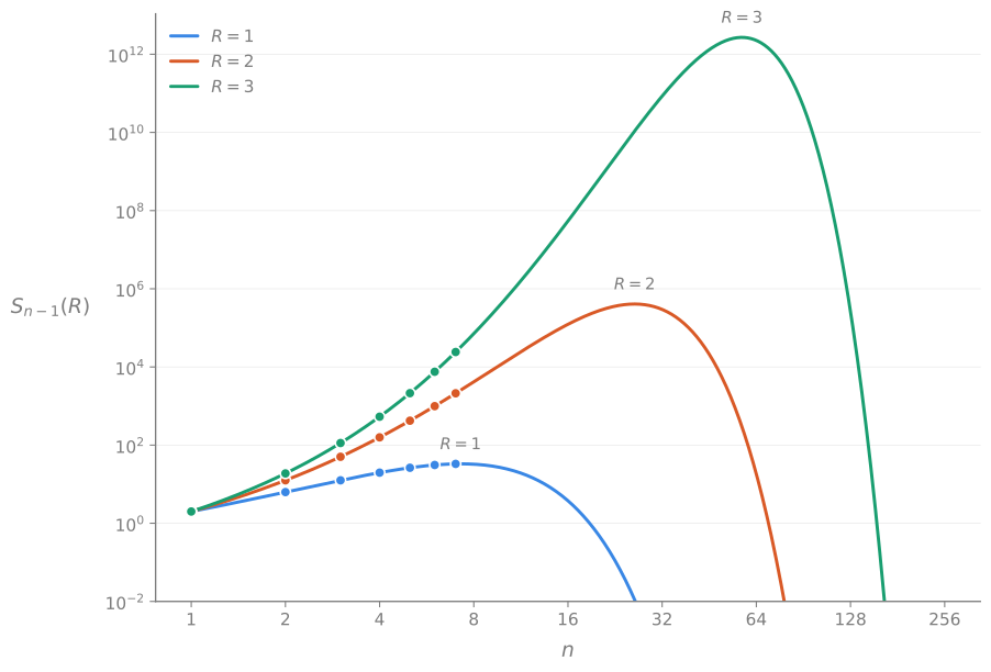
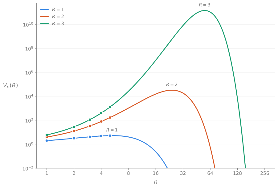
<p>Note that the unit $n$-ball volume peaks at $n=5$, while the unit $(n-1)$-sphere volume peaks at $n=7$ (i.e., with the $6$-sphere). Similar to the $n$-ball volume, increasing the radius only prolongs the inevitable.</p>

<figure>
  <center>
  <img src="/assets/blog/high-dimensional-space/the-surface-of-the-n-ball/surface-vs-dimension-log-multi.svg" alt="The volume of the sphere against dimension for multiple radii." />
  <figcaption><small><i>Plotting the hypervolume of the $(n-1)$-sphere against $n$ for multiple $R$.</i></small></figcaption>
  </center>
</figure>

<p>It’s still quite surprising, but not as much as before given that it’s basically the same argument as the $n$-ball.</p>

<h2 id="the-equator-phenomenon">The equator phenomenon</h2>

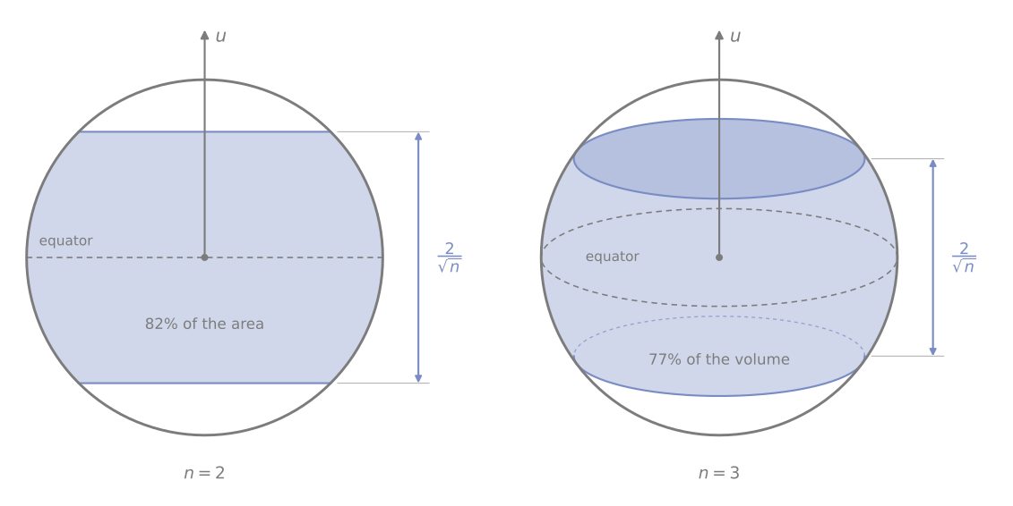
<p>The principle holds here for the surface as well, but I want to look at this topic through the perspective of the volume of the $n$-ball. I think the general idea and a similar bound come from <a class="citation" href="#ball1997elementary">(Ball, 1997)</a>.</p>

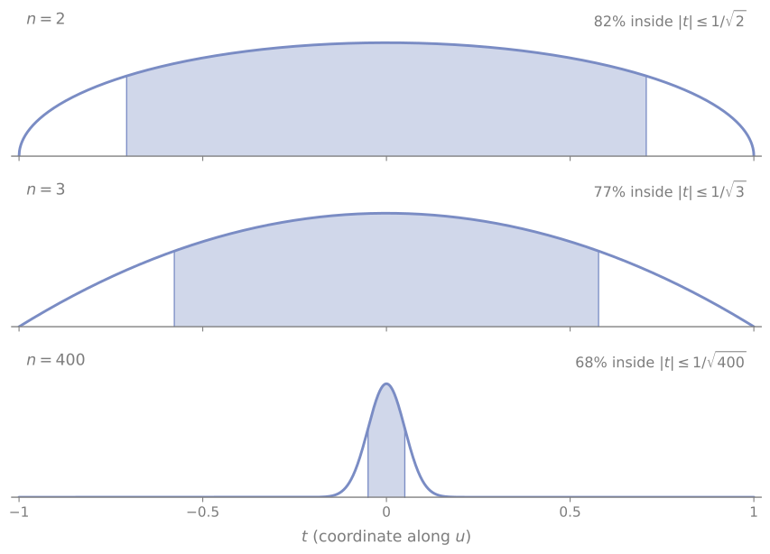
<p>Consider the unit $n$-ball centered in the origin. Pick any direction $\mathbf{u}$, and consider the normal hyperplane to that direction passing through the origin: that is the equator. If we consider a band of width $2/\sqrt{n}$ around this equator, what is the fraction of the volume of the $n$-ball within this band?</p>

<p>Here’s how it looks for 2D and 3D:</p>

<figure>
  <center>
  <img src="/assets/blog/high-dimensional-space/the-surface-of-the-n-ball/equator-band-pair.svg" alt="Volume of the equator band for 2D and 3D." />
  <figcaption><small><i>Plotting the equator band for the $2$-ball and $3$-ball.</i></small></figcaption>
  </center>
</figure>

<p>The band stands out relatively wide and as we increase the dimension, both the width of the band, as well as the ratio of the volume of the equator band to the unit ball start decreasing. But they don’t decrease in the same manner.</p>

<hr />

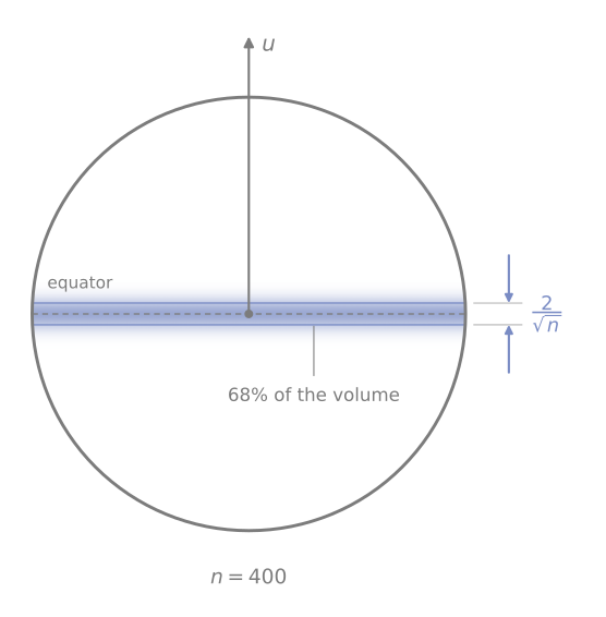
<p>Let’s try to visualize what happens when we increase the dimension, such as $n = 400$.
Even though we can’t directly visualize a $400$-ball, we can show its 2D projection while trying to accurately represent the approximate density of the ball at each point while moving along the direction of $\mathbf{u}$:</p>

<figure>
  <center>
  <img src="/assets/blog/high-dimensional-space/the-surface-of-the-n-ball/disk-equator-band-density.svg" alt="Volume of the equator band for a 400-ball." />
  <figcaption><small><i>Visualizing the equator band for the $400$-ball. Note that the shading is only meaningful along $\mathbf{u}$. Not to be confused with a literal 2D projection of the $400$-ball, which would just look like a small blob at the center about $1/\sqrt{n}$ wide.</i></small></figcaption>
  </center>
</figure>

<p>That looks quite unbelievable! It is fascinating how this thin equator band contains $\approx 68.3\%$ of the total volume of the $n$-ball, given that we can repeat it along any random direction and still its corresponding equator band will have the same percentage of the total volume. They all look like they share the “center” section, but let’s also not forget that the volume of the $n$-ball is also concentrated near the surface of the sphere, the center has basically no volume.</p>

<p>What is more interesting is that as we further increase $n$, the band grows thinner and thinner, while the volume ratio of the equator band to the unit ball stays $\approx 68.3\%$.</p>

<details open="" class="callout">
  <summary><b>Why?</b></summary>

  <p>Let’s use our cross-section machinery from the volume post: consider the unit ball (and the equator band) as a stack of $(n-1)$-dimensional balls along the direction vector $\mathbf{u}$, with varying radii $r_t = \sqrt{1 - t^2}$.</p>

  <p>The practical result is that at each point $t$ along the direction of $\mathbf{u}$, the density of the ball scales with $V_{n-1}(r_t)$. To see this, we use $V_{n}(R) = C_{n}R^{n}$:</p>

\[\begin{align}
V_{n-1}(\sqrt{1-t^2})
 &amp;= C_{n-1} \left( \sqrt{1-t^2} \right)^{n-1} \\
 &amp;= C_{n-1} (1 - t^2)^{(n-1)/2}.
\end{align}\]

  <p>Normalizing this by the unit ball volume $V_{n}(1)$ and integrating along the entire ball gives us $1$ per the cross-section formula from the previous post.</p>

\[\begin{align}
\int_{-1}^{1}\frac{V_{n-1}(\sqrt{1-t^2})}{V_{n}(1)}\,dt &amp;= \int_{-1}^{1}\frac{C_{n-1} (1-t^2)^{(n-1)/2}\,dt}{C_{n}\cdot 1^{n}} \\
&amp;= \int_{-1}^{1}\underbrace{\frac{C_{n-1}}{C_{n}}\cdot(1-t^2)^{(n-1)/2}}_{p(t)}\,dt.
\end{align}\]

  <p>Since $\frac{C_{n-1}}{C_n}$ is constant, this shows that the probability density function $p(t)$ scales with</p>

\[(1-t^2)^{(n-1)/2}.\]

  <h4 id="why-specifically-0683">Why specifically 0.683?</h4>

  <p>We have to look at the volume of the equator band compared to the volume of the unit $n$-ball.</p>

  <p>The ratio of the two volumes in $n$ dimensions, $\rho_{n}$, is equal to</p>

\[\begin{align}
\rho_{n} &amp;= \frac{\int_{-1/\sqrt{n}}^{1/\sqrt{n}}V_{n-1}(r_{t})\,dt}{V_{n}(1)} \\
     &amp;= \frac{\int_{-1/\sqrt{n}}^{1/\sqrt{n}}\frac{\pi^{(n-1)/2}}{\Gamma((n-1)/2 + 1)}\left(\sqrt{1-t^2}\right)^{n-1}\,dt}{\frac{\pi^{n/2}}{\Gamma(n/2 + 1)}} \\
     &amp;= \frac{\frac{\pi^{(n-1)/2}}{\Gamma((n-1)/2 + 1)}\int_{-1/\sqrt{n}}^{1/\sqrt{n}}\left(1-t^2\right)^{(n-1)/2}\,dt}{\frac{\pi^{n/2}}{\Gamma(n/2 + 1)}} \\
     &amp;= \frac{\pi^{(n-1)/2}}{\pi^{n/2}} \cdot \frac{\Gamma(n/2 + 1)}{\Gamma((n-1)/2 + 1)} \cdot 2 \int_{0}^{1/\sqrt{n}}(1-t^2)^{(n-1)/2}\,dt \\
     &amp;= \frac{2}{\sqrt{\pi}}\cdot \frac{\Gamma(n/2 + 1)}{\Gamma((n-1)/2 + 1)} \cdot \int_{0}^{1/\sqrt{n}}(1-t^2)^{(n-1)/2}\,dt.
\end{align}\]

  <p>This two-part form doesn’t simplify any further, but taking the limit $n \to \infty$ allows us to progress with the parts individually. I was stuck on this part for some time on these limits, and Claude helped with the following parts:</p>

  <p>First, taking the limit properly for these two needs the following adjustment:</p>

\[\rho_n = \sqrt{\frac{2}{\pi}}\cdot
\underbrace{\frac{\Gamma(n/2+1)}{\sqrt{n/2}\,\Gamma((n-1)/2+1)}}_{A_n}\cdot
\underbrace{\sqrt{n}\int_{0}^{1/\sqrt{n}}(1-t^2)^{(n-1)/2}\,dt}_{B_n}.\]

  <p>Now we look at them individually.</p>

  <ul>
    <li>For $A_{n}$, we have the ratio of Gamma functions resulting in</li>
  </ul>

\[\lim_{n\to\infty}A_{n} = 1.\]

  <p>This is shown in <a href="#appendix">the appendix</a>.</p>

  <ul>
    <li>For $B_{n}$, we first substitute $t = u / \sqrt{n}$ to get</li>
  </ul>

\[B_{n} = \sqrt{n}\int_{0}^{1/\sqrt{n}}(1-t^2)^{(n-1)/2}\,dt = \int_{0}^{1}\left(1-\frac{u^2}{n}\right)^{(n-1)/2}\,du.\]

  <p>We then look at $\lim_{n\to\infty}B_{n}$. The integrand $(1-u^2/n)^{(n-1)/2}$ is bounded and converges for every $u$ on $[0, 1]$, so by the dominated convergence theorem we can take the limit inside the integral and apply the identity $\lim_{n\to\infty}(1 + a/n)^{n} = e^{a}$:</p>

\[\begin{align}
\lim_{n\to\infty}B_{n} &amp;= \lim_{n\to\infty}\int_{0}^{1}\left(1-\frac{u^2}{n}\right)^{(n-1)/2}\,du \\
  &amp;=\int_{0}^{1}\lim_{n\to\infty}\left[\left(1-\frac{u^2}{n}\right)^{n}\right]^{1/2}\cdot \left(1-\frac{u^2}{n}\right)^{-1/2}\,du \\
  &amp;= \int_{0}^{1}\left(e^{-u^2}\right)^{1/2}\cdot1^{-1/2}\,du \\
  &amp;= \int_{0}^{1}e^{-u^2/2}\,du.
\end{align}\]

  <hr />

  <p>So, the product as $n\to\infty$ is then the product of these limits:</p>

\[\begin{align}
\lim_{n\to\infty}\rho_{n} &amp;= \sqrt{\frac{2}{\pi}} \cdot 1 \cdot \int_{0}^{1}e^{-u^2/2}\,du \\
 &amp;= \sqrt{\frac{2}{\pi}}\int_{0}^{1}e^{-u^2/2}\,du.
\end{align}\]

  <p>Finally, we substitute $u = \sqrt{2}\,s$ to transform the integral into the form of the <a href="https://en.wikipedia.org/wiki/Error_function">error function</a>:</p>

\[\begin{align}
\lim_{n\to\infty}\rho_{n} &amp;= \sqrt{\frac{2}{\pi}}\cdot \sqrt{2} \cdot \int_{0}^{1/\sqrt{2}}e^{-s^2}\,ds \\
&amp;= \mathrm{erf}(1/\sqrt{2}) \\
&amp;\approx 0.683. \tag*{$\Box$}
\end{align}\]

  <p>We used $\mathrm{erf}(x) = \frac{2}{\sqrt{\pi}}\int_{0}^{x}e^{-s^2}\,ds$ in the last part above.</p>

</details>

<hr />

<p>Another intuitive way to visualize this is to directly look at the marginal distribution of the points of the $n$-ball onto the 1D line of the direction vector $\mathbf{u}$:</p>

<figure>
  <center>
  <img src="/assets/blog/high-dimensional-space/the-surface-of-the-n-ball/equator-band-marginal-density.svg" alt="Marginal density through the direction vector axis." />
  <figcaption><small><i>Plotting the marginal density of the $n$-ball through projection onto $\mathbf{u}$.</i></small></figcaption>
  </center>
</figure>

<p>The marginal distributions above show how the distribution of points along a random direction changes as $n$ increases. For high dimensions, $68.3\%$ of points lie within the band of $2/\sqrt{n}$ width. This is slightly intuitive when we consider that most individual coordinates for randomly sampled points on the sphere should have magnitude close to $1/\sqrt{n}$, which is one of the core ideas for a following post on angles in high-dimensional space.</p>

<div class="callout">

  <p>In summary, this ~30-year-old quote from <a class="citation" href="#ball1997elementary">(Ball, 1997)</a> is still relevant:</p>

  <blockquote>
    <p>So the volume of the ball concentrates close to any subspace of dimension $n−1$. This would seem to suggest that the volume concentrates near the centre of the ball, where the subspaces all meet. But, on the contrary, it is easy to see that, if $n$ is large, most of the volume of the ball lies near its surface. In objects of high dimension, measure tends to concentrate in places that our low-dimensional intuition considers small.</p>
  </blockquote>

</div>

<h2 id="a-practical-note-on-why-the-surface">A practical note on “Why the surface?”</h2>

<p>One thing that frequently pops up in machine learning is to normalize high-dimensional samples from a dataset for reasons like measuring cosine similarity or retrieving samples. Given a sample $\mathbf{x} \in \mathbf{X} \subset \mathbb{R}^d$, L2-normalizing the sample $\mathbf{x} \leftarrow \frac{\mathbf{x}}{ \lVert \mathbf{x} \rVert}$ puts it on the surface of the $d$-dimensional unit ball, i.e., the $(d-1)$-dimensional unit sphere.</p>

<p>Representation spaces are commonly $512$, $768$ or $1024$-dimensional for stuff like word embeddings (see <a href="/blog/2026/09/02/building-wordsim/">a previous post</a> for an example) and vision-language embeddings (e.g., CLIP, SigLIP), where both the volume and surface area are practically in the <em>funky</em> high-dimensional regime, looking at the volume scaling graph.</p>

<p>Hopefully, now we have a bit more insight towards the fact that this $(d-1)$-sphere does not have our 2D or 3D expectations in appearance, distribution, or concentration of volume.</p>

<h2 id="appendix">Appendix</h2>

<h3 id="the-limit-of-the-gamma-ratio">The limit of the Gamma ratio</h3>

<p>Recall that we’re concerned with the limit</p>

\[\begin{align}
\lim_{n\to\infty}A_{n} &amp;= \lim_{n\to\infty}\frac{\Gamma(n/2 + 1)}{\Gamma((n-1)/2 + 1)\sqrt{n/2}}.
\end{align}\]

<p>Let $g(x) = \frac{\Gamma(x+1)}{\Gamma(x + \frac{1}{2})}$. We’re going to need $g(n/2)$. We have the very useful property of</p>

\[g(x)g(x-\frac{1}{2}) = \frac{\Gamma(x+1)}{\Gamma(x + \frac{1}{2})} \cdot
  \frac{\Gamma(x+\frac{1}{2})}{\Gamma(x)} = \frac{\Gamma(x+1)}{\Gamma(x)} = x,\]

<p>using $\Gamma(z+1)=z\,\Gamma(z)$.</p>

<p>Similarly, we see that</p>

\[g(x)g(x+\frac{1}{2}) = x + \frac{1}{2}.\]

<p>The function $g(x)$ is monotonically increasing, since $\log\Gamma(x)$ is convex (a commonly known property). Thus we have</p>

\[g(x - \frac{1}{2}) \leq g(x) \leq g(x + \frac{1}{2}).\]

<p>Multiply everything by $g(x) &gt; 0$:</p>

\[g(x)g(x - \frac{1}{2}) \leq g^2(x) \leq g(x)g(x + \frac{1}{2}).\]

<p>Using the identities we just proved:</p>

\[x \leq g^2(x) \leq x + \frac{1}{2},\]

<p>then take the square root:</p>

\[\sqrt{x} \leq g(x) \leq \sqrt{x + \frac{1}{2}}.\]

<p>Divide by $\sqrt{x}$ to get</p>

\[1 \leq \frac{g(x)}{\sqrt{x}} \leq \sqrt{1 + \frac{1}{2x}},\]

<p>and finally substitute $x = n/2$ to recover $A_{n}$:</p>

\[1 \leq \frac{g(n/2)}{\sqrt{n/2}} = \frac{\Gamma(n/2 + 1)}{\Gamma((n-1)/2 + 1)\sqrt{n/2}} = A_{n} \leq \sqrt{1 + \frac{1}{n}}.\]

<p>All that’s left is to look at the limit as $n\to\infty$. We have</p>

\[\lim_{n\to\infty} 1 = \lim_{n\to\infty}\sqrt{1 + \frac{1}{n}} = 1.\]

<p>Therefore, by the squeeze theorem we have</p>

\[\lim_{n\to\infty}A_{n} = 1. \tag*{$\Box$}\]]]></content><author><name>Çağrı Eser</name></author><summary type="html"><![CDATA[I talk about the surface of the n-ball, perhaps better referred to as the (n-1)-sphere.]]></summary><media:thumbnail xmlns:media="http://search.yahoo.com/mrss/" url="https://cagrislist.org/assets/blog/thumbs/the-surface-of-the-n-ball.png" /><media:content medium="image" url="https://cagrislist.org/assets/blog/thumbs/the-surface-of-the-n-ball.png" xmlns:media="http://search.yahoo.com/mrss/" /></entry><entry><title type="html">The volume of the n-ball</title><link href="https://cagrislist.org/blog/2026/09/20/the-volume-of-the-n-ball/" rel="alternate" type="text/html" title="The volume of the n-ball" /><published>2026-09-20T00:00:00+00:00</published><updated>2026-09-20T00:00:00+00:00</updated><id>https://cagrislist.org/blog/2026/09/20/the-volume-of-the-n-ball</id><content type="html" xml:base="https://cagrislist.org/blog/2026/09/20/the-volume-of-the-n-ball/"><![CDATA[<p class="callout"><small> This is the second entry in the
<a href="/blog/2026/09/16/a-leap-into-high-dimensional-space/">high-dimensional space blog series</a>.
</small></p>

<p>In <a href="/blog/2026/09/16/the-volume-of-the-four-ball/">the previous post</a>, we were able to calculate the (hyper-)volume of the $4$-dimensional ball of radius $R$ as</p>

\[V_{4}(R) = \frac{1}{2}\pi^2 R^{4}.\]

<p>How do we extend this to any $n$-dimensional ball? How does the volume change with $n$? The $n$-ball contains many super interesting mysteries.</p>

<p>What follows next is some math, then a couple of counterintuitive properties. For example:</p>

<ul>
  <li>We show that the volume first increases, and then <strong>plummets to zero</strong> with increasing $n$.</li>
  <li>Nearly all of the $n$-ball’s volume concentrates in an arbitrarily thin shell near the boundary as $n$ increases.</li>
</ul>

<p>Let’s dive in!</p>

<h2 id="intermediate-properties-of-the-n-ball">Intermediate properties of the $n$-ball</h2>

<p>Before we tackle the question head-on, we need some intermediate results. Many of these results come from building up the $n$-ball from the $(n-1)$-ball.</p>

<h3 id="a-recurrence-between-v_nr-and-v_n-1r">A recurrence between $V_{n}(R)$ and $V_{n-1}(R)$</h3>

<p>Recall that we showed</p>

\[V_{4}(R) = \int_{-R}^{R} \frac{4}{3}\pi r_{w}^{3}\,dw,\]

<p>where we defined $r_{w} = \sqrt{R^2 - w^2}$ as the radius of the cross-section along the $w$ dimension, and it had a corresponding hypervolume of $V_{3}(r_{w}) = \frac{4}{3}\pi r_{w}^3$.</p>

<p>This extends to any dimension $n$. The cross-sections of the $n$-balls that we integrate to find the hypervolume are themselves $(n-1)$-balls, so in general we obtain the following expression for the $n$-dimensional hypervolume:</p>

\[\boxed{V_{n}(R) = \int_{-R}^{R} V_{n-1}\left(\sqrt{R^2 - x^2}\right)\,dx}. \tag{1}
\label{eq:eq1}\]

<p>This is a very promising recurrence relation, as it allows us to find the general formula to the volume of the $n$-ball.</p>

<h3 id="mining-the-recurrence-for-simplicity">Mining the recurrence for simplicity</h3>

<p>The first instinct we have with a recurrence relation like \eqref{eq:eq1} is to see if unrolling reveals any useful properties. Our efforts are rewarded with the following result:</p>

\[\boxed{V_{n}(R) = 2\pi \int_{0}^{R}tV_{n-2}(t)\,dt}. \tag{2}
\label{eq:eq2}\]

<details open="" class="callout">
  <summary><b>Why?</b></summary>

  <p><strong>Proof.</strong> In the integral of \eqref{eq:eq1}, we see a term $V_{n-1}\left(\sqrt{R^2 - x^2}\right)$. But what is this term? Let’s use the same definition, now over a different integration variable $y$:</p>

\[\begin{align*}
V_{n-1}\left(\sqrt{R^2 - x^2}\right) &amp;= \int_{-\sqrt{R^2 - x^2}}^{\sqrt{R^2 - x^2}} V_{n-2}\left(\sqrt{\left(\sqrt{R^2 - x^2}\right)^2 - y^2}\right)\,dy \\
    &amp;=\int_{-\sqrt{R^2 - x^2}}^{\sqrt{R^2-x^2}}V_{n-2}\left(\sqrt{R^2 - x^2 - y^2}\right)\,dy. \tag{$\ast$}
    \label{eq:eqstar}
\end{align*}\]

  <p>Putting \eqref{eq:eqstar} in \eqref{eq:eq1}:</p>

\[V_{n}(R) = \int_{-R}^{R}\int_{-\sqrt{R^2 - x^2}}^{\sqrt{R^2-x^2}}V_{n-2}\left(\sqrt{R^2 - x^2 - y^2}\right)\,dy\,dx.\]

  <p>Notice that our integration axes trace out the disk $x^2 + y^2 \leq R^2$. Can we use polar coordinates? Yes, we can.</p>

  <p>Letting $x^2 + y^2 = r^2$ with $x = r\cos\theta$ and $y=r\sin\theta$, we can express this last integral as a double integral over the disk:</p>

\[\begin{align}
V_{n}(R) &amp;= \int_{0}^{2\pi}\int_{0}^{R}V_{n-2}\left( \sqrt{R^2 - r^2} \right)r\,dr\,d\theta \\
         &amp;= 2\pi \int_{0}^{R}V_{n-2}\left( \sqrt{R^2 - r^2} \right)\,r\,dr,
\end{align}\]

  <p>making use of $dx\,dy=r\,dr\,d\theta$. We then employ a change in variables</p>

\[\begin{align}
t^2 &amp;= R^2 - r^2 \\
2t\,dt &amp;= -2r\,dr
\end{align}\]

  <p>and obtain with slight adjustments the result:</p>

\[\begin{align}
V_{n}(R) &amp;= 2\pi \int_{R}^{0}-t\,V_{n-2}(t)\,dt \\
         &amp;= \boxed{2\pi \int_{0}^{R}tV_{n-2}(t)\,dt}. \tag*{$\Box$}
\end{align}\]

</details>

<p>This lets us “skip” a dimension for a practically much easier integral, which will be useful later.</p>

<h3 id="a-general-form-of-the-n-ball-volume">A general form of the $n$-ball volume</h3>

<p>As we saw with previous volume formulas $2R, \pi\,R^2, \frac{4\pi}{3}R^3$, it looks like all of the $n$-ball hypervolumes follow a specific sequence. It turns out that we can also formalize this as</p>

\[\begin{equation}
\boxed{V_{n}(R) = C_{n}R^{n}}, \tag{3}
\label{eq:eq3}
\end{equation}\]

<p>where $C_{n} = V_{n}(1)$ is the volume of the unit ball!</p>

<details open="" class="callout">
  <summary><b>Why?</b></summary>

  <p><strong>Proof.</strong> Our observation hints towards induction. We oblige, and use induction to show that with the base case $V_{1}(R) = 2R$, the general relation $V_{n}(R) = C_{n}R^{n}$ holds. By the inductive property we have</p>

\[\begin{align}
V_{n+1}(R) &amp;= \int_{-R}^{R} V_{n}\left(\sqrt{R^2 - x^2}\right)\,dx \tag{from (1)} \\
           &amp;= \int_{-R}^{R} C_{n} \left(\sqrt{R^2 - x^2}\right)^{n}\,dx \tag{by induction}\\
           &amp;= C_{n} \int_{-R}^{R} (R^2 - x^2)^{n/2}\,dx.
\end{align}\]

  <p>We now substitute in</p>

\[\begin{align}
    x &amp;= R\sin\theta, \\
    dx &amp;= R\cos\theta\,d\theta.
\end{align}\]

  <p>Now,</p>

\[\begin{align}
V_{n+1}(R) 
    &amp;= C_{n} \int_{-\pi/2}^{\pi/2}(R^2 - R^2\sin^2\theta)^{n/2}R\cos\theta\,d\theta \\
    &amp;= C_{n} \int_{-\pi/2}^{\pi/2}(R^2 (1 - \sin^2\theta))^{n/2}R\cos\theta\,d\theta \\
    &amp;= C_{n} \int_{-\pi/2}^{\pi/2}(R^2 \cos^2\theta)^{n/2}R\cos\theta\,d\theta \\
    &amp;= C_{n} R^{n+1} \int_{-\pi/2}^{\pi/2}\cos^{n+1}\theta\,d\theta.
\end{align}\]

  <p>In particular, the integral $\int_{-\pi/2}^{\pi/2}\cos^{n+1}\theta\,d\theta$ is a Wallis integral which comes up a lot in calculations about the $n$-ball. We don’t need to look further into it now, the important thing here is that it is a constant that can be absorbed by $C_{n+1}$.</p>

  <p>Thus, we have already shown that by defining</p>

\[C_{n+1} = C_{n}\int_{-\pi/2}^{\pi/2}\cos^{n+1}\theta\,d\theta,\]

  <p>we arrive at $V_{n+1}(R) = C_{n+1} R^{n+1}$ as promised. We also note that with $V_{n}(R) = C_{n}R^{n}$, letting $R=1$ directly gives us</p>

\[V_{n}(1) = C_{n} 1^{n} = C_{n},\]

  <p>which proves the second part of the claim.</p>

</details>

<h3 id="deriving-the-general-recurrence-relation">Deriving the general recurrence relation</h3>

<p>Combining \eqref{eq:eq2} with \eqref{eq:eq3} gives us a new recurrence relation:</p>

\[\begin{equation}
\boxed{V_{n}(R) = \frac{2\pi R^{2}}{n}V_{n-2}(R)}. \tag{4}
\label{eq:eq4}
\end{equation}\]

<details open="" class="callout">
  <summary><b>Why?</b></summary>

  <p>We’re going to plug in the new form, $V_{n}(R) = C_{n}R^{n}$ into \eqref{eq:eq2}.</p>

\[\begin{align}
V_{n}(R)
    &amp;= 2\pi \int_{0}^{R}tV_{n-2}(t)\,dt \\
    &amp;= 2\pi \int_{0}^{R}tC_{n-2}t^{n-2}\,dt \\
    &amp;= 2\pi\,C_{n-2}\int_{0}^{R}t^{n-1}\,dt \\
    &amp;= 2\pi\,C_{n-2}\left(\frac{t^{n}}{n}\right)\Big\vert_{0}^{R} \\
    &amp;= \frac{2\pi}{n}C_{n-2}R^{n} \\
    &amp;= \frac{2\pi R^2}{n}V_{n-2}(R).
\end{align}\]

  <p>Recalling that $V_{n}(R) = C_{n}R^{n}$ by \eqref{eq:eq3}, note that we also find</p>

\[C_{n} = \frac{2\pi}{n}C_{n-2}. \tag*{$\Box$}\]

</details>

<h2 id="the-closed-form-of-the-n-ball-volume-formula">The closed-form of the $n$-ball volume formula</h2>

<p>Eq. \eqref{eq:eq4} gives us the insight we need to instantly calculate the volume of the $n$-ball.</p>

<p>Intuitively, it says that whenever we increase the dimension by two (from $n-2$ to $n$), we scale the previous volume by $\frac{2\pi R^2}{n}$. We can obtain the formula for the $n$ case by collecting these multipliers with each added dimension.</p>

<p>The resulting $n$-ball volume formula is then</p>

\[\boxed{V_{n}(R) = \frac{\pi^{n/2}}{\Gamma(n/2 + 1)}R^{n}}, \tag{5}\]

<p>where $\Gamma(z)$ is the Gamma function.</p>

<details open="" class="callout">
  <summary><b>Why?</b></summary>

  <p>We have to look at odd and even cases separately and apply \eqref{eq:eq4} starting from the base cases.</p>

  <h4 id="odd-powers-of-n">Odd powers of $n$</h4>

  <p>For odd powers $n = 2k +1$, we start from $V_{1}(R) = 2R$ and move towards $V_{2k+1}(R)$.</p>

\[\begin{align}
V_{2k+1}(R)
    &amp;= V_{1}(R) \times \underbrace{\frac{2\pi R^2}{3} \times \frac{2\pi R^2}{5} \times \cdots \times \frac{2\pi R^2}{2k + 1}}_{k \, \text{terms}} \\
    &amp;= 2R \times \frac{\left(2\pi R^2\right)^{k}}{3 \cdot 5 \cdots (2k+1)} \\
    &amp;= \frac{2 (2\pi)^{k}}{(2k+1)!!} R^{2k+1}.
\end{align}\]

  <p>Here, we used the double factorial, defined as $(2k +1)!! = 1 \cdot 3 \cdot 5 \cdots (2k+1)$.</p>

  <h4 id="even-powers-of-n">Even powers of $n$</h4>

  <p>For the even case $n = 2k$, we have the much more intuitive</p>

\[\begin{align}
V_{2k}(R)
    &amp;= V_{2}(R) \times \underbrace{\frac{2\pi R^2}{4} \times \frac{2\pi R^2}{6} \times \cdots \times \frac{2\pi R^2}{2k}}_{(k-1) \, \text{terms}} \\
    &amp;= \frac{\pi R^2 \times (2\pi R^2)^{k-1}}{2^{k-1} (1\cdot2\cdots k)} \\
    &amp;= \frac{2^{k-1}\pi^{k}R^{2k}}{2^{k-1}k!} \\
    &amp;= \frac{\pi^{k}}{k!}R^{2k}.
\end{align}\]

  <h4 id="unifying-the-odd-and-even-cases">Unifying the odd and even cases</h4>

  <p>This is the hardest part.</p>

  <p>At first glance, the odd and even cases seem to be quite different. However, we know by \eqref{eq:eq1} that each volume for the $n$ case actually builds up from the previous $(n-1)$ case in the exact same manner.</p>

  <p>We need some utility that unifies the two cases, and it specifically needs to align the factorial part: The even formula $V_{2k}(R) = \frac{\pi^{k}}{k!}R^{2k}$ looks great, but we can’t substitute $2k \rightarrow 2k+1$ because the factorial is only defined for positive integers. The answer is the Gamma function, $\Gamma(z)$.</p>

  <hr />

  <p>The <a href="https://en.wikipedia.org/wiki/Gamma_function">Gamma function</a> has two properties that we will use. The first is that it extends the factorial to non-integer values, with</p>

\[\begin{align}
\Gamma(z + 1) &amp;= z \Gamma(z) &amp;\text{for } z &gt; 0, \\
\Gamma(z+1) &amp;= z! &amp;\text{for }z \in \mathbb{Z}^{+}.
\end{align}\]

  <p>The other property is that for $z=\frac{1}{2}$ it is equal to</p>

\[\Gamma(\frac{1}{2}) = \sqrt{\pi}.\]

  <p>With these two properties, we can use the Gamma function to unify the two cases with</p>

\[V_{n}(R) = \frac{\pi^{n/2}}{\Gamma(\frac{n}{2} + 1)}R^{n}.\]

  <p><strong>Proof.</strong> For the odd case $n = 2k+1$, we have</p>

\[\begin{align}
V_{2k+1}(R)
    &amp;= \frac{\pi^{(2k+1)/2}}{\Gamma(\frac{2k+1}{2} + 1)}R^{2k+1} \\
    &amp;= \frac{\pi^{k}\pi^{1/2}}{\Gamma(\frac{2k+1}{2} + 1)}R^{2k+1} \\
    &amp;= \frac{\pi^{k}\sqrt{\pi}}{\sqrt{\pi} \cdot \frac{1}{2} \cdot \frac{3}{2} \cdots \frac{2k+1}{2}}R^{2k+1} \\
    &amp;= \frac{2^{k+1}\pi^{k}}{\underbrace{1\cdot3\cdot5\cdots(2k+1)}_{k+1\,\mathrm{terms}}}R^{2k+1} \\
    &amp;= \frac{2(2\pi)^{k}}{(2k+1)!!}R^{2k+1}.
\end{align}\]

  <p>Similarly, for the even case,</p>

\[\begin{align}
V_{2k}(R)
    &amp;= \frac{\pi^{2k/2}}{\Gamma(\frac{2k}{2} + 1)}R^{2k} \\
    &amp;= \frac{\pi^{k}}{\Gamma(k+1)}R^{2k} \\
    &amp;= \frac{\pi^k}{k!}R^{2k}.
\end{align}\]

  <p>So, the unifying equation for the volume of the $n$-ball using $\Gamma(z)$ explains both odd and even cases of $n$.</p>

</details>

<p>For even values $n = 2k$ we have the simpler</p>

\[\boxed{V_{2k}(R) = \frac{\pi^{k}}{k!}R^{2k}}, \tag{6}\]

<p>which is very handy in examining scaling for the $n$-ball.</p>

<p>Here are some example values for the volume of the $n$-ball, up to $n=9$.</p>

<table class="table-centered table-alt-cols">
  <thead>
    <tr>
      <th style="text-align: right">$n$</th>
      <th style="text-align: right">$V_n(R)$</th>
      <th style="text-align: right">$n$</th>
      <th style="text-align: right">$V_n(R)$</th>
      <th style="text-align: right">$n$</th>
      <th style="text-align: right">$V_n(R)$</th>
    </tr>
  </thead>
  <tbody>
    <tr>
      <td style="text-align: right">1</td>
      <td style="text-align: right">$2R$</td>
      <td style="text-align: right">4</td>
      <td style="text-align: right">$\dfrac{\pi^2}{2}R^4$</td>
      <td style="text-align: right">7</td>
      <td style="text-align: right">$\dfrac{16\pi^3}{105}R^7$</td>
    </tr>
    <tr>
      <td style="text-align: right">2</td>
      <td style="text-align: right">$\pi R^2$</td>
      <td style="text-align: right">5</td>
      <td style="text-align: right">$\dfrac{8\pi^2}{15}R^5$</td>
      <td style="text-align: right">8</td>
      <td style="text-align: right">$\dfrac{\pi^4}{24}R^8$</td>
    </tr>
    <tr>
      <td style="text-align: right">3</td>
      <td style="text-align: right">$\dfrac{4\pi}{3}R^3$</td>
      <td style="text-align: right">6</td>
      <td style="text-align: right">$\dfrac{\pi^3}{6}R^6$</td>
      <td style="text-align: right">9</td>
      <td style="text-align: right">$\dfrac{32\pi^4}{945}R^9$</td>
    </tr>
  </tbody>
</table>

<p>But a table is hard to look at.</p>

<h2 id="analyzing-the-n-ball">Analyzing the $n$-ball</h2>

<p>We did all of the hard work, let’s see some visuals!</p>

<p>For a moment, let’s think of the $n$-cube: for a side length of $\ell$ its volume is $\ell^{n}$.</p>
<ul>
  <li>if the side length is $\ell = 1$, then the volume is $1\times1\times\cdots\times1=1$.</li>
  <li>If the side length is $\ell &lt; 1$, then with each dimension we’re multiplying with a value smaller than $1$, which means as $n \rightarrow \infty$ we have $\mathrm{volume} \rightarrow 0$. The decrease is exponential in $n$ due to $\ell^n$.</li>
  <li>If the side length is $\ell &gt; 1$, then with each dimension we have $\mathrm{volume} \rightarrow \infty$ as $n \rightarrow \infty$. The increase is exponential in $n$.</li>
</ul>

<p>So, with this in mind: how does the $n$-ball change? Recall the formula is</p>

\[V_{n}(R) = \frac{\pi^{n/2}}{\Gamma(n / 2 + 1)}R^{n}.\]

<p>With $R = 1$, the volume increases as we increase $n$:</p>

<figure>
  <center>
  <img src="/assets/blog/high-dimensional-space/2026-09-19-the-volume-of-the-n-ball/volume-vs-dimension-n-5.svg" alt="Volume against dimension, up to n = 5." />
   <figcaption><small><i>Plotting $V_{n}(1)$ against $n$.</i></small></figcaption>
   </center>
</figure>

<p>… until we reach $n = 5$. After that, the volume decreases. And not only does it decrease, it decreases <strong>superexponentially</strong>, faster than any exponential function!</p>

<figure>
  <center>
  <img src="/assets/blog/high-dimensional-space/2026-09-19-the-volume-of-the-n-ball/volume-vs-dimension-log.svg" alt="Volume against dimension, smoothly up to n = 128." />
   <figcaption><small><i>Plotting $V_{n}(1)$ against $n$, smoothly until $n = 128$.</i></small></figcaption>
   </center>
</figure>

<p>This looks like a very thrilling rollercoaster ride. Not only is the volume asymptotically going to $0$, but beyond a very reasonable $n$ value it is practically zero as well!</p>

<p>For $n=16$ we have</p>

\[V_{16}(1) = \frac{\pi^8}{8!} \approx 0.235,\]

<p>and for $n = 32$ we have</p>

\[V_{32}(1) = \frac{\pi^{16}}{16!} \approx 4.30307 \times 10^{-6} = 0.0000043.\]

<p>For most applications, that is practically zero.</p>

<div class="callout">
  <h3 id="why-does-it-decrease-so-fast-and-why-n5">Why does it decrease so fast, and why $n=5$?</h3>
  <p>The reason for this is the ratio between the numerator and the denominator, more easily seen in the even case $n=2k$:</p>

\[V_{2k}(R) = \frac{\pi^{k}}{k!}R^{2k}.\]

  <p>For the unit $n$-ball with $n=2k$, whenever we “add two dimensions”, we multiply the previous volume by $\frac{\pi}{k}$. When starting out, multiplying by $\pi \approx 3.14$ is more impactful than dividing by $k=1, k=2, …$, but after $k &gt; \pi$ the denominator quickly dominates.</p>

  <p>In the asymptotic case, we know that</p>

\[\lim_{k\rightarrow\infty}\frac{\pi^{k}}{k!} = 0.\]

  <hr />

  <p>If we treat the formula as a continuous function, the absolute peak is at $n \approx 5.26$.</p>

</div>

<h3 id="what-about-a-larger-ball">What about a larger ball?</h3>

<p>We can try to beat this process by looking at a slightly larger ball, since we would also scale the volume by $R^{n}$. Instead of $R=1$, let’s take $R = 2$ or $R=3$: that should give us a $2^{n}$ and $3^{n}$ scale factor, respectively.</p>

<figure>
  <center>
  <img src="/assets/blog/high-dimensional-space/2026-09-19-the-volume-of-the-n-ball/volume-vs-dimension-log-multi.svg" alt="Volume against dimension with multiple R, smoothly up to n = 256." />
   <figcaption><small><i>Plotting $V_{n}(R)$ against $n$, smoothly until $n = 256$.</i></small></figcaption>
   </center>
</figure>

<p>It does not help. There is no escaping the rollercoaster that is the volume of the $n$-ball.</p>

<div class="callout">
  <p>The volume of the $n$-ball increases, and then goes to zero faster than any exponential function.</p>
</div>

<h2 id="where-is-the-volume-of-the-n-ball">Where is the volume of the $n$-ball?</h2>

<p>Consider a very thin shell of the unit $n$-ball, obtained by drawing the $n$-ball with unit radius $R = 1$ and then putting a slightly smaller $n$-ball of radius $0.98R$. What is the ratio of the volume of the inner ball to the outer ball?</p>

<figure>
  <center>
  <img src="/assets/blog/high-dimensional-space/2026-09-19-the-volume-of-the-n-ball/nested-balls-n123.svg" alt="Nested n-balls." />
   <figcaption><small><i>Nested $n$-balls of radius $R$ and $0.98R$.</i></small></figcaption>
   </center>
</figure>

<p>In the figure above, you can barely see the gap between the inner and the outer $n$-balls.</p>

<ul>
  <li>For $n = 1$, we have</li>
</ul>

\[\frac{V_{1}(0.98R)}{V_{1}(R)} = \frac{2\cdot 0.98R}{2\cdot R} = 0.98.\]

<ul>
  <li>For $n = 2$, we have</li>
</ul>

\[\frac{V_{2}(0.98R)}{V_{2}(R)} = \frac{\pi(0.98R)^2}{\pi R^2} = (0.98)^2 = 0.9604.\]

<ul>
  <li>For $n = 3$, we have</li>
</ul>

\[\frac{V_{3}(0.98R)}{V_{3}(R)} = \frac{\frac{4\pi}{3}(0.98R)^3}{\frac{4\pi}{3} R^3} = (0.98)^3 \approx 0.9412.\]

<p>… you get the picture. We start off pretty strong, and visually we can see that most of the volume of the $n$-ball is inside the volume of the smaller $n$-ball.</p>

<p>However, by $n=128$ the ratio is now</p>

\[\frac{V_{128}(0.98R)}{V_{128}(R)} \approx 0.0753.\]

<p>For a $128$-ball, approximately $92.47\%$ of the outer ball’s volume is concentrated in the thin shell!</p>

<p>We can express the specific ratio for some $n$ and $R$ with</p>

\[\begin{align}
1 - \frac{V_{n}(0.98R)}{V_{n}(R)} &amp;= 1 - \frac{C_{n}(0.98R)^{n}}{C_{n}R^n} \\
    &amp;= 1 - (0.98)^{n}.
\end{align}\]

<p>As $n \rightarrow \infty$, we see that the ratio becomes $1$. There is basically no volume unless you are near the boundary.</p>

<div class="callout">
  <p>With increasing $n$, the volume of the $n$-ball is concentrated in an arbitrarily thin shell near the boundary of the ball.</p>
</div>

<h2 id="sampling-from-the-unit-n-ball">Sampling from the unit $n$-ball</h2>

<p>We end this one with sampling points in the unit $n$-ball. In my case, it was quite peculiar when I had to deal with it recently.</p>

<p>How do you sample from the $n$-ball of radius $R$? Suppose you have access to the uniform distribution and the normal distribution.</p>

<p>One idea is rejection sampling. It’s very fast and intuitive, let’s look at the 2D case.</p>

<ol>
  <li>We sample $x$ and $y$ such that $x,y \sim \mathcal{U}[-1, 1]$ are from the uniform distribution.</li>
  <li>We calculate $r = \sqrt{x^2 + y^2}$.</li>
  <li>If $r \leq R$ we keep the sample (it’s in the disk), otherwise we reject it.</li>
</ol>

<p>Here’s how it looks for 1000 candidate $(x, y)$ pairs in step (1).</p>
<figure>
  <center>
  <img src="/assets/blog/high-dimensional-space/2026-09-19-the-volume-of-the-n-ball/rejection-sampling-disk.svg" alt="Rejection sampling on the disk." />
   <figcaption><small><i>Rejection sampling on the unit disk.</i></small></figcaption>
   </center>
</figure>

<p>Empirically, $773 / 1000 = 0.773$ were in the disk. On paper, we expect around</p>

\[\frac{\pi\cdot1^2}{2 \times 2} = \frac{\pi}{4} \approx 0.785\]

<p>of sampled points to be valid samples, or</p>

\[1000\cdot\frac{1}{0.785} \approx 1273\]

<p>candidates to successfully sample 1000 points inside the unit disk. As you might expect this doesn’t scale to higher dimensions very well.</p>

<p>For $n=20$ we have</p>

\[\frac{V_{20}(1)}{2^{20}} = \frac{\pi^{10} / 10!}{1048576} \approx 2.46 \times 10^{-8},\]

<p>or approximately</p>

\[1000 \cdot \frac{1}{2.46 \times 10^{-8}} \approx 4 \times 10^{10},\]

<p>or $40000000000$ candidate points just to perhaps sample 1000 points inside the unit $20$-ball. <a class="citation" href="#hicks1959efficient">(Hicks &amp; Wheeling, 1959)</a> states that generating acceptable random points from the $20$-cube would have yielded roughly “40 points per century”, albeit on an ancient 704 program.</p>

<p>Rejection sampling is basically impossible for higher dimensions, due to its inefficiency.</p>

<h3 id="the-gaussian-trick">The Gaussian trick</h3>

<p>I’m not sure who the entire process is attributed to, although the normalized Gaussian idea appears to be from <a class="citation" href="#muller1959note">(Muller, 1959)</a>. This is actually from the same journal issue as the Hicks and Wheeling quote above, and Muller also credits <a href="https://en.wikipedia.org/wiki/George_W._Brown_(computer_scientist)">George W Brown</a> on suggesting the method.</p>

<p>The trick works in three steps.</p>

<ol>
  <li>We start by sampling $\mathbf{g} \sim \mathcal{N}(0, I_{n})$, the $n$-dimensional Gaussian distribution. We then normalize it as $\mathbf{v} = \frac{\mathbf{g}}{\lVert \mathbf{g} \rVert}$.</li>
</ol>

<div class="callout">

  <h4 id="why-the-gaussian">Why the Gaussian?</h4>

  <p>The short answer is that the Gaussian is rotationally symmetric, so normalizing the points gives us a uniform distribution over the unit $n$-sphere (the boundary of the $n$-ball).</p>

  <figure>
  <center>
  <img src="/assets/blog/high-dimensional-space/2026-09-19-the-volume-of-the-n-ball/gaussian-sampling-disk.svg" alt="Normalizing the Gaussian distribution." />
   <figcaption><small><i>Normalizing the Gaussian distribution gives us a uniform distribution on the boundary of the unit $n$-ball.</i></small></figcaption>
   </center>
</figure>

</div>

<p>Now, we have to disperse the points on the $n$-sphere with the appropriate radius distribution of the $n$-ball.</p>

<ol start="2">
  <li>We sample $u \sim \mathcal{U}[0, 1]$ and let $r = u^{1/n}$.</li>
</ol>

<div class="callout">

  <p>We want uniform sampling within the ball. This means that when sampling some $r$, we want the probability $r \leq \rho$ for some $\rho \in (0, 1]$ to be equal to the ratio of the volumes between $V_{n}(\rho)$ and $V_{n}(1)$ (this is the CDF).</p>

\[P(r \leq \rho) = \frac{V_{n}(\rho)}{V_{n}(1)} = \frac{C_{n}\rho^{n}}{C_{n}1^n} = \rho^{n}.\]

  <p>Inverting this CDF gives us $r = u^{1/n}$ for uniform sampling within the ball.</p>

  <hr />

  <p><small>
(<em>Cagri’s note</em>: I initially tried $r \sim \mathcal{U}[0, 1]$ to get a “uniform” radius distribution; however that doesn’t work. It assigns too much towards the center of the ball, whereas we just learned that volume concentrates at the boundary. Scaling by volume is the way to go.)
</small></p>

</div>

<p>The product $r \cdot \mathbf{v}$ already gives us a random uniform sample from the unit $n$-ball.</p>

<ol start="3">
  <li>Scale it by multiplying with $R$ to randomly sample from the $n$-ball with radius $R$ instead.</li>
</ol>

<p>After all three steps, the product $R\cdot r \cdot \mathbf{v}$ gives us a uniformly sampled random variable in the $n$-ball with radius $R$, quite efficiently and without any rejection sampling.</p>

<h2 id="closing-remarks">Closing remarks</h2>

<p>There are many more properties about the $n$-ball that I want to talk about, and this is only scratching the surface. We saw a couple major properties in this post.</p>

<ul>
  <li>
    <p>The closed-form volume formula can be derived from the cross-section integral, as we showed in the first section.</p>
  </li>
  <li>
    <p>The volume of the $n$-ball is a rollercoaster that briefly rises before plummeting to its doom (zero).</p>
  </li>
  <li>
    <p>As $n$ increases, the volume increasingly concentrates near the boundary of the $n$-ball.</p>
  </li>
  <li>
    <p>It’s slightly difficult to sample from at first glance, but efficient with some tricks.</p>
  </li>
</ul>

<p>Next time, I’ll talk about the surface of the $n$-ball and an alternative formulation for the volume.</p>]]></content><author><name>Çağrı Eser</name></author><summary type="html"><![CDATA[I derive and talk about the hypervolume of the $n$-dimensional ball, in this series on high-dimensional spaces.]]></summary><media:thumbnail xmlns:media="http://search.yahoo.com/mrss/" url="https://cagrislist.org/assets/blog/thumbs/the-volume-of-the-n-ball.png" /><media:content medium="image" url="https://cagrislist.org/assets/blog/thumbs/the-volume-of-the-n-ball.png" xmlns:media="http://search.yahoo.com/mrss/" /></entry><entry><title type="html">A leap into high dimensional space [series]</title><link href="https://cagrislist.org/blog/2026/09/16/a-leap-into-high-dimensional-space/" rel="alternate" type="text/html" title="A leap into high dimensional space [series]" /><published>2026-09-16T00:00:00+00:00</published><updated>2026-09-16T00:00:00+00:00</updated><id>https://cagrislist.org/blog/2026/09/16/a-leap-into-high-dimensional-space</id><content type="html" xml:base="https://cagrislist.org/blog/2026/09/16/a-leap-into-high-dimensional-space/"><![CDATA[<blockquote>
  <p>“To deal with hyper-planes in a 14-dimensional space, visualize a 3-D space and say ‘fourteen’ to yourself very loudly. Everyone does it.”</p>

  <p>Geoffrey Hinton</p>
</blockquote>

<p>Humans are really good at visualizing one, two, and three dimensions. Unfortunately, this doesn’t scale past three very well<sup id="fnref:1"><a href="#fn:1" class="footnote" rel="footnote" role="doc-noteref">1</a></sup>. What’s more interesting is that some of the intuition that we have for 2D and 3D <em>really</em> doesn’t extend to higher dimensions as we might initially expect.</p>

<hr />

<p>Here is the series in chronological order (to be updated with new entries over time):</p>

<ol>
  <li>
    <p><a href="/blog/2026/09/16/the-volume-of-the-four-ball/">The volume of the $4$-ball</a></p>
  </li>
  <li>
    <p><a href="/blog/2026/09/20/the-volume-of-the-n-ball/">The volume of the $n$-ball</a></p>
  </li>
  <li>
    <p><a href="/blog/2026/09/25/the-surface-of-the-n-ball/">The surface of the $n$-ball</a></p>
  </li>
  <li>
    <p><a href="/blog/2026/10/09/the-n-dimensional-gaussian/">The $n$-dimensional Gaussian distribution</a></p>
  </li>
</ol>

<hr />

<div class="footnotes" role="doc-endnotes">
  <ol>
    <li id="fn:1">
      <p>Although there are apparently methods to visualize a 4D space, I’m not sure how accessible it is for everyone and how effective it is. Reading about it feels like people describing going on spiritual trips. <a href="#fnref:1" class="reversefootnote" role="doc-backlink">&#8617;</a></p>
    </li>
  </ol>
</div>]]></content><author><name>Çağrı Eser</name></author><summary type="html"><![CDATA[I briefly explore various geometric concepts in higher dimensions.]]></summary><media:thumbnail xmlns:media="http://search.yahoo.com/mrss/" url="https://cagrislist.org/favicon/android-chrome-512x512.png" /><media:content medium="image" url="https://cagrislist.org/favicon/android-chrome-512x512.png" xmlns:media="http://search.yahoo.com/mrss/" /></entry><entry><title type="html">The volume of the 4-ball</title><link href="https://cagrislist.org/blog/2026/09/16/the-volume-of-the-four-ball/" rel="alternate" type="text/html" title="The volume of the 4-ball" /><published>2026-09-16T00:00:00+00:00</published><updated>2026-09-16T00:00:00+00:00</updated><id>https://cagrislist.org/blog/2026/09/16/the-volume-of-the-four-ball</id><content type="html" xml:base="https://cagrislist.org/blog/2026/09/16/the-volume-of-the-four-ball/"><![CDATA[<p class="callout"><small> This is the first entry in the
<a href="/blog/2026/09/16/a-leap-into-high-dimensional-space/">high-dimensional space blog series</a>.
</small></p>

<p>In the familiar low-dimensional spaces around us, we have a way to quantify how much room something takes up.</p>

<p>In one dimension it is the <strong>length</strong>, in two dimensions it is the <strong>area</strong>, and in 3D we have the <strong>volume</strong>.</p>

<p>What do we call this notion with higher dimensions? It’s called the <strong>hypervolume</strong><sup id="fnref:1"><a href="#fn:1" class="footnote" rel="footnote" role="doc-noteref">1</a></sup>.</p>

<p>The two most basic geometric objects we have are cubes and balls. The unit cube is not as interesting at first, because it always occupies $1 \times 1 \times … \times 1 = 1$ unit of space regardless of its dimension.</p>

<figure>
  <center>
  <img src="/assets/blog/high-dimensional-space/unit-square-cube.svg" alt="Simple squares and cubes." />
  <figcaption><small><i>The unit square and unit cube, with area 1 and volume 1 respectively.</i></small></figcaption>
  </center>
</figure>

<p>In contrast, the ball is a lot more fun.</p>

<h2 id="some-definitions">Some definitions</h2>

<p>We denote by $V_{n}(R)$ the hypervolume of the <em>$n$-ball</em>, which is the generalization of a ball in $n$-dimensional space.</p>

<p>The closed $n$-ball with center $\mathbf{x} \in \mathbb{R}^{n}$ and radius $R$ is defined as</p>

\[B(\mathbf{x}; R) := \lbrace \mathbf{y} \in \mathbb{R}^{n} \mid d(\mathbf{x}, \mathbf{y}) \leq R \rbrace.\]

<p>So it’s just all of the points around a point $\mathbf{x}$ that are at most $R$ units away from $\mathbf{x}$ based on some distance metric $d$.</p>

<p>In this post we are concerned with Euclidean distance $d(\mathbf{x}, \mathbf{y}) = \lVert\mathbf{x} - \mathbf{y} \rVert_{2}$, and the ball centered at the origin (so $\mathbf{x} = 0$). Thus, our ball definition simplifies to just a set containing points $\mathbf{p} = (p_{1}, …, p_{n})$, such that</p>

\[p_{1}^{2} + p_{2}^{2} + ... + p_{n}^{2} \leq R^{2}.\]

<p>That’s all nice, but how do we compute the hypervolume of an $n$-ball?</p>

<p>Naturally, we start from $n=1$ and build up.</p>

<h3 id="1-ball">$1$-ball</h3>

<p>The $1$-ball of radius $R$ is an interval $[-R, R]$ around the origin. 
It has a length of $R - (-R) = 2R$, which is also its 1-dimensional hypervolume $V_{1}(R) = 2R$.</p>

<figure>
  <center>
  <img src="/assets/blog/high-dimensional-space/ball-1d.svg" alt="A 1D ball." />
  <figcaption><small><i>A one-dimensional ball of radius $R$.</i></small></figcaption>
  </center>
</figure>

<p>It is not very round, is it? However, it is in fact the roundest thing one can ever find in 1D.</p>

<h3 id="2-ball">$2$-ball</h3>

<p>The closed $2$-ball is our good old friend, the disk. From school we know by heart that it has area equal to $V_{2}(R) = \pi R^{2}$.</p>

<figure>
  <center>
  <img src="/assets/blog/high-dimensional-space/ball-2d.svg" alt="A 2D ball." />
  <figcaption><small><i>A two-dimensional ball of radius $R$.</i></small></figcaption>
  </center>
</figure>

<h3 id="3-ball">$3$-ball</h3>

<p>The $3$-ball is the most intuitive one, in that it is what you would call a ball in everyday life. It has volume equal to</p>

\[V_{3}(R) = \frac{4}{3}\pi R^{3}.\]

<p>We again learn it by heart during school.</p>

<hr />

<p>However, in multivariate calculus we are able to show it with the aid of the following idea: a ball is a vertically stacked arrangement of two-dimensional disks:</p>

<figure>
  <center>
  <img src="/assets/blog/high-dimensional-space/ball-3d-slices.svg" alt="A 3D ball." />
  <figcaption><small><i>A $3$-ball of radius $R$, thought of as a stack of disks.</i></small></figcaption>
  </center>
</figure>

<p>With our knowledge of integrals, we know that we can represent this infinite sum of disks as an integral as we move in the $z$-axis. However, we also notice that each disk has its own radius that depends on the particular value of $z$. Geometrically, we can show it as this:</p>

<figure>
  <center>
  <img src="/assets/blog/high-dimensional-space/disk-triangle-3d.svg" alt="Close-up on the 3D ball." />
  <figcaption><small><i>Zooming in on a disk of the $3$-ball.</i></small></figcaption>
  </center>
</figure>

<p>For each disk with height $h$, the radius is</p>

\[r_{h} = \sqrt{R^2 - h^2}, \tag{1}\]

<p>and its area is $\pi r_{h}^2$.  Thus, the total volume is</p>

\[V_{3}(R) = \int_{-R}^{R}\pi r_{h}^{2}\,dh = \frac{4}{3}\pi R^{3}.\]

<details open="" class="callout">
  <summary><b>Calculating the integral</b></summary>

  <p>No tricks needed here, we can just evaluate it head on:</p>

\[\begin{align}
V_{3}(R) &amp;= \int_{-R}^{R}\pi r_{h}^{2} \,dh \\
         &amp;= \int_{-R}^{R}\pi\left(\sqrt{R^{2} - h^{2}}\right)^{2}\,dh \tag{from (1)} \\
         &amp;= \pi\int_{-R}^{R}(R^2 - h^2) \,dh \\
         &amp;= \pi \left(R^2 h - \frac{h^3}{3} \right) \Big\vert_{-R}^{R} \\
         &amp;= \pi (2R^3 - 2\frac{R^3}{3}) \\
         &amp;= \frac{4\pi}{3}R^{3}. \tag*{$\Box$}
\end{align}\]

</details>

<p>Which brings us to the case of the 4-ball. What’s one more dimension?</p>

<h3 id="4-ball">4-ball</h3>

<p>Unfortunately, we can’t visualize the $4$-dimensional ball.</p>

<p>We don’t know what a 4-dimensional ball looks like; all we know is that it is composed of points $\mathbf{p} = (x, y, z, w)$ such that</p>

\[\lVert \mathbf{p} \rVert _{2}^2 = x^2 + y^2 + z^2 + w^2 \leq R^{2}.\]

<p>How can we calculate the (hyper-)volume of this thing that we can’t visualize?</p>

<p>To progress, we actually have to go backwards.</p>

<h2 id="retracing-our-steps">Retracing our steps</h2>

<p>Upon closer inspection, we can see that our stack-of-disks explanation for the $3$-ball is just as applicable for the two-dimensional disk as well. The disk is a stack of horizontal intervals, which are actually $1$-balls as we discussed earlier!</p>

<figure>
  <center>
  <img src="/assets/blog/high-dimensional-space/disk-2d-slices.svg" alt="2D disk as a stack of 1D intervals." />
  <figcaption><small><i>The disk is a vertical stack of $1$-balls.</i></small></figcaption>
  </center>
</figure>

<p>Again, each $1$-ball has some radius $r$ that depends on the current $y$, with ${r_{y} = \sqrt{R^2 - y^2}}$ as $y$ moves along $[-R, R]$. They have a length of $2 r_{y}$, which we’ll sum up to obtain the area.</p>

<p>The integral here is actually slightly trickier than the 3-dimensional case, but it turns out that</p>

\[V_{2}(R) = \int_{-R}^{R}2 r_{y}\,dy = \pi R^2,\]

<p>as we would expect.</p>

<details open="" class="callout">
  <summary><b>Calculating the integral</b></summary>

  <p>We start off with:</p>

\[\begin{align}
V_{2}(R) &amp;= \int_{-R}^{R}2 r_{y} \, dy \\
         &amp;= 2\int_{-R}^{R}\left(\sqrt{R^{2} - y^{2}}\right) dy \\
         &amp;= 4\int_{0}^{R}\left(\sqrt{R^{2} - y^{2}}\right) dy. \tag{by symmetry}
\end{align}\]

  <p>We then apply the change of variables</p>

\[\begin{align}
 y &amp;= R \sin\theta, \\
 dy &amp;= R \cos\theta \, d\theta.
\end{align}\]

  <p>which also means the limits of integration $(0, R)$ change to $(0, \pi / 2)$.</p>

  <p>Now,</p>

\[\begin{align}
V_{2}(R) &amp;= 4\int_{0}^{\pi / 2}\sqrt{R^2 - (R\sin\theta)^2}R\cos\theta \, d\theta \\
         &amp;= 4R^2\int_{0}^{\pi / 2}\sqrt{1 - \sin^{2}\theta} \cos\theta \, d\theta \\
         &amp;= 4R^2\int_{0}^{\pi / 2}\sqrt{\cos^{2}\theta} \cos\theta \, d\theta \\
         &amp;= 4R^2\int_{0}^{\pi / 2}\cos^{2}\theta \, d\theta. \tag{$\cos\theta \geq 0$}
\end{align}\]

  <p>It is known that $\int_{0}^{\pi / 2}\cos^{2}\theta \, d\theta = \frac{\pi}{4}$, but it is also easy to derive (see <a href="#appendix">the appendix</a>). Plugging it in we have</p>

\[\begin{align}
V_{2}(R) &amp;= 4R^2 \cdot \frac{\pi}{4} \\
         &amp;= \pi R^2. \tag*{$\Box$}
\end{align}\]

</details>

<hr />

<p>This even works for the $1$-ball (interval) as well, if we consider it to be a stack of points (zero-dimensional balls), each of volume $V_{0} = 1$. The integral for the 1D case is just</p>

\[\begin{align}
V_{1}(R) &amp;= \int_{-R}^{R}1\, dx \\
         &amp;= 2R.
\end{align}\]

<hr />

<p>To summarize, we see that constructing the $n$-dimensional ball is possible by vertically stacking $(n-1)$-dimensional balls along the new dimension and summing up their respective hypervolume.</p>

<h2 id="back-to-the-4-ball">Back to the $4$-ball</h2>

<p>Before we continue, I want to sketch one aspect of the $4$-ball.</p>

<ul>
  <li>When we slice the 1D interval on $x$, we get a point.</li>
  <li>When we slice the disk along the new dimension $y$, we get an interval (a $1$-ball).</li>
  <li>When we slice the $3$-ball along the new dimension $z$, we get a disk (a $2$-ball).</li>
</ul>

<p>That means that when we slice the $4$-ball, we’re going to get a $3$-ball when we look at the cross-section.</p>

<p>This is my best attempt at actually visualizing this idea, slicing across the new dimension $w$:</p>

<figure>
  <center>
  <img src="/assets/blog/high-dimensional-space/four-ball-overlap-sqrt.svg" alt="The cross-sections of a 4-ball." />
  <figcaption><small><i>The cross-sections of the $4$-ball are $3$-balls (shown only for $w \geq 0$).</i></small></figcaption>
  </center>
</figure>

<p>Let’s not be fooled, these balls are actually not intersecting. All of the cross-sections live in their own three-dimensional hyperplane with a constant $w$. None of them share any points, and they have zero thickness<sup id="fnref:2"><a href="#fn:2" class="footnote" rel="footnote" role="doc-noteref">2</a></sup> along $w$. It’s also incredibly interesting how the cross-sections stay quite large for most of the way, and only collapse near $w=R$.</p>

<p>This idea of summing up cross-sections is called <a href="https://en.wikipedia.org/wiki/Cavalieri%27s_principle">Cavalieri’s principle</a>, and the rigorous version is known as <a href="https://en.wikipedia.org/wiki/Fubini's_theorem">Fubini’s theorem</a>.</p>

<h3 id="the-4-ball-revisited">The $4$-ball, revisited</h3>

<p>We’re back here again, but equipped with new machinery. Our idea is simple: Given a fixed $w$, the points $\mathbf{p} = (x, y, z, w)$ are in the cross-section</p>

\[x^2 + y^2 + z^2 \leq R^2 - w^2 \tag{2}\]

<p>of the $4$-ball centered at the origin with radius $R$. We know that (2) is the definition of a $3$-ball with radius $r_{w} = \sqrt{R^2 - w^2}$ and volume $\frac{4}{3}\pi r_{w}^3$. We can sum their volumes together over $w$ to obtain our prize, the hypervolume of the $4$-ball.</p>

<p>We express this as the integral</p>

\[V_{4}(R) = \int_{-R}^{R} \frac{4}{3}\pi r_{w}^{3}\,dw\]

<p>which turns out to be… with drum roll please…</p>

\[\boxed{V_{4}(R) = \frac{1}{2}\pi^2 R^{4}}.\]

<details open="" class="callout">
  <summary><b>Calculating the integral</b></summary>

  <p>Our approach is similar to the 2-dimensional case, which actually isn’t surprising.</p>

  <p>We start off with:</p>

\[\begin{align}
V_{4}(R) &amp;= \int_{-R}^{R}\frac{4}{3}\pi r_{w}^3 \, dw \\
         &amp;= \frac{4\pi}{3}\int_{-R}^{R}\left(\sqrt{R^{2} - w^{2}}\right)^{3} \, dw \\
         &amp;= \frac{8\pi}{3}\int_{0}^{R}\left(R^{2} - w^{2}\right)^{3/2} dw. \tag{by symmetry}
\end{align}\]

  <p>We again apply the change of variables</p>

\[\begin{align}
 w &amp;= R \sin\theta, \\
 dw &amp;= R \cos\theta \, d\theta.
\end{align}\]

  <p>and that also means the limits of integration $(0, R)$ change to $(0, \pi / 2)$.</p>

  <p>Now,</p>

\[\begin{align}
V_{4}(R) &amp;= \frac{8\pi}{3}\int_{0}^{\pi / 2}\left(R^2 - R^2\sin^2\theta\right)^{3/2} R\cos\theta \, d\theta \\
         &amp;= \frac{8\pi}{3}R^{4}\int_{0}^{\pi / 2} \left(\cos^{2}\theta\right)^{3/2} \cos\theta \, d\theta \\
         &amp;= \frac{8\pi}{3}R^{4}\int_{0}^{\pi / 2} \cos^{4}\theta \, d\theta. \tag{$\cos\theta \geq 0$}
\end{align}\]

  <p>It is known that $\int_{0}^{\pi / 2}\cos^{4}\theta \, d\theta = \frac{3\pi}{16}$, and we derive it in <a href="#appendix">the appendix</a> to keep things short. Plugging it in, we arrive at</p>

\[\begin{align}
V_{4}(R) &amp;= \frac{8\pi}{3}R^{4} \cdot \frac{3\pi}{16} \\
         &amp;= \frac{1}{2}\pi^2 R^4. \tag*{$\Box$}
\end{align}\]

</details>

<hr />

<p>What’s really nice is that this method extends to the $5$-ball, a $100$-ball, or any arbitrary $n$-ball hypervolume by summing up cross-sections of $(n-1)$-balls.</p>

<p>Its recursive nature also allows us to obtain closed-form solutions for any high-dimensional ball. We’ll explore general properties of the $n$-ball in the next post.</p>

<h2 id="appendix">Appendix</h2>

<h4 id="deriving-int_0pi--2cos2theta--dtheta">Deriving $\int_{0}^{\pi / 2}\cos^2\theta \, d\theta$</h4>

<p>This one is kinda pretty. Substituting $\theta \to \frac{\pi}{2} - \theta$, we have the useful</p>

\[\int_0^{\pi/2}\cos^2\theta\, d\theta = \int_0^{\pi/2}\sin^2\theta\, d\theta.\]

<p>Over the same interval we sum them together:</p>

\[2\int_{0}^{\pi/2}\cos^2\theta\,d\theta = \int_0^{\pi/2}(\cos^2\theta + \sin^2\theta)\,d\theta = \frac{\pi}{2},\]

<p>making use of $\sin^2\theta + \cos^2 \theta = 1$.</p>

<p>Therefore,</p>

\[\int_{0}^{\pi / 2} \cos^2 \theta \, d\theta = \frac{1}{2}\cdot\frac{\pi}{2} = \frac{\pi}{4}. \tag{3}\]

<hr />

<h4 id="deriving-int_0pi--2cos4thetadtheta">Deriving $\int_{0}^{\pi / 2}\cos^{4}\theta\,d\theta$</h4>

<p>Note that we have  $\cos^{4}\theta = \cos^{2}\theta(1-\sin^{2}\theta)$, meaning that we can write everything as</p>

\[\int_{0}^{\pi/2}\cos^4\theta\,d\theta = \int_{0}^{\pi/2}\cos^2\theta\,d\theta - \int_{0}^{\pi/2}\cos^2\theta\sin^2\theta\,d\theta.\]

<p>The first term, the one with $\cos^{2}\theta$, is exactly what we want. We showed that it is equal to $\frac{\pi}{4}$ in the previous section.</p>

<p>For the second term, we can use the double angle identity $\sin\theta\cos\theta = \frac{1}{2}\sin 2\theta$:</p>

\[\int_{0}^{\pi / 2}\cos^2\theta\sin^2\theta\, d\theta = \frac{1}{4}\int_{0}^{\pi / 2}\sin^2 2\theta\, d\theta.\]

<p>Applying the change of variables $u = 2\theta$, so that $d\theta = \frac{1}{2}\,du$ and the limits become $[0, \pi]$:</p>

\[\frac{1}{4}\int_{0}^{\pi / 2}\sin^2 2\theta \, d\theta = \frac{1}{8}\int_{0}^{\pi} \sin^2 u \, du.\]

<p>We can reuse our previous result. Since $\sin^2(\pi - u) = \sin^2 u$, the halves $[0, \frac{\pi}{2}]$ and $[\frac{\pi}{2}, \pi]$ contribute equally, so</p>

\[\begin{align}
\int_{0}^{\pi}\sin^2 u \, du &amp;= \int_{0}^{\pi/2}\sin^2 u \, du + \int_{\pi/2}^{\pi}\sin^2 u \, du \\
                             &amp;= 2\int_{0}^{\pi/2}\sin^2 u \, du \\
                             &amp;= 2 \cdot \frac{\pi}{4} \\ 
                             &amp;= \frac{\pi}{2},
\end{align}\]

<p>where we used $\int_0^{\pi/2}\sin^2 \theta\, d\theta = \int_0^{\pi/2}\cos^2 \theta \, d\theta = \frac{\pi}{4}$ from (3). Therefore</p>

\[\int_{0}^{\pi /2} \sin^{2}2\theta \, d\theta = \frac{1}{2} \cdot \frac{\pi}{2} = \frac{\pi}{4}.\]

<p>Putting it all together:</p>

\[\begin{align}
\int_{0}^{\pi / 2}\cos^4 \theta\, d\theta
  &amp;= \int_{0}^{\pi / 2}\cos^2 \theta \, d\theta - \frac{1}{4}\int_{0}^{\pi /2} \sin^{2}2\theta\,d\theta \\
  &amp;=\frac{\pi}{4} - \frac{1}{4}\cdot\frac{\pi}{4} \\
  &amp;= \frac{\pi}{4} - \frac{\pi}{16} \\
  &amp;= \frac{3\pi}{16}. \tag*{$\Box$}
\end{align}\]

<hr />

<div class="footnotes" role="doc-endnotes">
  <ol>
    <li id="fn:1">
      <p>More formally, the hypervolume of a subset of $\mathbb{R}^{n}$ corresponds to its $n$-dimensional Lebesgue measure. <a href="#fnref:1" class="reversefootnote" role="doc-backlink">&#8617;</a></p>
    </li>
    <li id="fn:2">
      <p>It might be more honest to draw them as flat disks when expanding towards $w$ to emphasize this, however then it looks just like the 3D case. Also, that would be worse as we’d be showing the cross-sections as disks rather than $3$-balls! <a href="#fnref:2" class="reversefootnote" role="doc-backlink">&#8617;</a></p>
    </li>
  </ol>
</div>]]></content><author><name>Çağrı Eser</name></author><summary type="html"><![CDATA[I talk about the (hyper-)volume of the four-dimensional ball, in this series on high-dimensional spaces.]]></summary><media:thumbnail xmlns:media="http://search.yahoo.com/mrss/" url="https://cagrislist.org/assets/blog/thumbs/the-volume-of-the-four-ball.png" /><media:content medium="image" url="https://cagrislist.org/assets/blog/thumbs/the-volume-of-the-four-ball.png" xmlns:media="http://search.yahoo.com/mrss/" /></entry><entry><title type="html">Building wordsim</title><link href="https://cagrislist.org/blog/2026/09/02/building-wordsim/" rel="alternate" type="text/html" title="Building wordsim" /><published>2026-09-02T00:00:00+00:00</published><updated>2026-09-02T00:00:00+00:00</updated><id>https://cagrislist.org/blog/2026/09/02/building-wordsim</id><content type="html" xml:base="https://cagrislist.org/blog/2026/09/02/building-wordsim/"><![CDATA[<p><small><em>Best viewed in dark mode.</em></small></p>

<p>It’s been a week or two since I launched <a href="https://cagrislist.org/projects/wordsim">wordsim</a>, and I’ve had a lot of questions from people on how and why it works behind the scenes. In this post, I want to expand on these topics and my own experience in building this simple but surprisingly addictive game.</p>

<p>In the first part, we’ll go over the fundamental concepts of representing words and determining word similarities. I want to go into details of representations with much more detail in a future post, but here I’ll try to keep the discussion here to a minimum.</p>

<p>Then, I’ll give a technical breakdown of how everything is implemented and how the pipeline works. We’ll have a short section on adapting the game to the Turkish language, and about some unexpected challenges in the process.</p>

<p>Let’s start!</p>

<figure>
  <center>
  <img src="/assets/blog/2026-09-02-building-wordsim/images/tr-umap.webp" alt="Teaser figure for Turkish word representations." />
  <figcaption><small><i>Teaser for what lies ahead for Turkish word representations.</i></small></figcaption>
  </center>
</figure>

<h2 id="about-wordsim-and-how-it-works">About wordsim, and how it works</h2>

<p>There comes a time for many people where they make a simple game about guessing words or numbers.
<code class="language-plaintext highlighter-rouge">wordsim</code> is such a game focusing on guessing a hidden word using semantic similarities.</p>

<p>It started as a spin-off of my curiosity in exploring how deep language models internally represent various concepts and the relations between these concepts. I had some prior experience in working with embeddings of vision-language models like CLIP <a class="citation" href="#radford2021learning">(Radford et al., 2021)</a>, or recently leveraging them for slightly more complex tasks such as <a href="https://arxiv.org/abs/2607.00777">jazz standard recognition</a>. I then wanted to explore the geometry of word embeddings.</p>

<h3 id="the-core-mechanism-of-word-similarity-games">The core mechanism of word similarity games</h3>

<p>This particular genre dates itself back to the childhood classic “hot or cold” guessing game, where one player hides an object within a room and guides another player to find that object using clues such as “cold” and “warm”. This idea naturally extends to a word guessing game: one player thinks of a word, and upon receiving a guess, gives clues about the semantic “closeness” of their guess until the word is eventually found. That is precisely how <code class="language-plaintext highlighter-rouge">wordsim</code> is played.</p>

<figure>
  <img src="/assets/blog/2026-09-02-building-wordsim/images/semantic.svg" alt="Conceptual hot-cold progression of words for the word 'sun'." />
  <center>
  <figcaption><small><i>Visualizations of closeness for the word "sun".</i></small></figcaption>
  </center>
</figure>

<p>Of course, implementing this idea is not nearly close to being a novel thought: looking for such a game leads one to games like <a href="https://contexto.me">Contexto</a>, the daily semantic-guessing game <a href="https://semantle.com">Semantle</a>, and many more implementations. I am not aware of any Turkish-focused word similarity game of this nature other than <code class="language-plaintext highlighter-rouge">wordsim</code> at the moment, so perhaps there is a small but unique contribution of the project there.</p>

<p>To successfully implement wordsim, conceptually we need two things:</p>

<ol>
  <li>A way to represent words.</li>
  <li>A way to compute similar words to a target word.</li>
</ol>

<p>Let’s start with item #2 first.</p>

<h3 id="thinking-about-word-similarities">Thinking about word similarities</h3>

<p>How does one determine which words are similar? Let’s start from some simple ideas:</p>

<ul>
  <li>
    <p>“forest” reminds us of “tree”, because forests are made of trees. Relations such as “has a”, “is a”, and words with the same or very similar meanings exhibit naturally strong similarity.</p>
  </li>
  <li>
    <p>There are multiple angles to approach a word. You can reach “earth” by starting from the solar system and the planets, as well as starting from seeds, farming and soil. Although they are seemingly unrelated paths, these two concepts should both lead to “earth” via increasing similarity.</p>
  </li>
  <li>
    <p>Similarity should be somewhat transitive: if we only report high similarity for immediate neighbors of a word, it’s very hard to reach that word from a random starting point. If the word is “egg”, then we expect “chicken” to be a very similar word, and “feather” to be similar to “chicken”. Thus, “egg” and “feather” should be somewhat similar as “chicken” is highly similar to both of them.</p>
  </li>
</ul>

<p>…and so on. We can’t establish all of these requirements by hand, as they would be too specific and brittle. We’d like to have a system that implicitly infers these kinds of relations.</p>

<p>Luckily for us, this is the natural area of language modeling in machine learning. With enough data and an appropriate model, we might be able to satisfy all of these requirements directly by learning them from the data.</p>

<hr />

<h3 id="how-do-we-represent-words">How do we represent words?</h3>

<p>At the most basic level we need to find a way to represent a word so that we can give it to a model. In natural language processing (NLP), the traditional way to do this was to build “one-hot encodings” for each word to give to a model:</p>

<ol>
  <li>Collect all words that you know from the text. Let’s say we collected 8 words, this is now our <code class="language-plaintext highlighter-rouge">vocabulary</code>.</li>
  <li>Give them a unique ordering, so that each word has its unique index.</li>
  <li>Represent a word by a series of 0s and 1s, such that only its unique index is 1 while all other entries are 0. This is called a “<a href="https://www.geeksforgeeks.org/machine-learning/ml-one-hot-encoding/">one-hot encoding</a>”.</li>
</ol>

<p>We can afford skipping grammatical details like word normalization, filtering, and out-of-dictionary words to simplify the general idea. Let’s go over a small example:</p>

<div class="language-python highlighter-rouge"><div class="highlight"><pre class="highlight"><code><span class="n">docs</span> <span class="o">=</span> <span class="p">[</span>
    <span class="p">[</span><span class="sh">'</span><span class="s">this</span><span class="sh">'</span><span class="p">,</span> <span class="sh">'</span><span class="s">is</span><span class="sh">'</span><span class="p">,</span> <span class="sh">'</span><span class="s">a</span><span class="sh">'</span><span class="p">,</span> <span class="sh">'</span><span class="s">dog</span><span class="sh">'</span><span class="p">],</span> <span class="c1"># an example sentence from the dataset
</span>    <span class="p">[</span><span class="sh">'</span><span class="s">cat</span><span class="sh">'</span><span class="p">,</span> <span class="sh">'</span><span class="s">and</span><span class="sh">'</span><span class="p">,</span> <span class="sh">'</span><span class="s">dog</span><span class="sh">'</span><span class="p">],</span>
    <span class="p">[</span><span class="sh">'</span><span class="s">a</span><span class="sh">'</span><span class="p">,</span> <span class="sh">'</span><span class="s">mouse</span><span class="sh">'</span><span class="p">],</span>
    <span class="p">[</span><span class="sh">'</span><span class="s">cat</span><span class="sh">'</span><span class="p">,</span> <span class="sh">'</span><span class="s">and</span><span class="sh">'</span><span class="p">,</span> <span class="sh">'</span><span class="s">mouse</span><span class="sh">'</span><span class="p">,</span> <span class="sh">'</span><span class="s">game</span><span class="sh">'</span><span class="p">]</span>
<span class="p">]</span>
<span class="n">words</span> <span class="o">=</span> <span class="nf">set</span><span class="p">()</span>
<span class="k">for</span> <span class="n">doc</span> <span class="ow">in</span> <span class="n">docs</span><span class="p">:</span>
    <span class="k">for</span> <span class="n">word</span> <span class="ow">in</span> <span class="n">doc</span><span class="p">:</span>
        <span class="n">words</span><span class="p">.</span><span class="nf">add</span><span class="p">(</span><span class="n">word</span><span class="p">)</span>
<span class="n">vocab</span> <span class="o">=</span> <span class="nf">sorted</span><span class="p">(</span><span class="nf">list</span><span class="p">(</span><span class="n">words</span><span class="p">))</span>
<span class="nf">print</span><span class="p">(</span><span class="n">vocab</span><span class="p">)</span> <span class="c1"># ['a', 'and', 'cat', 'dog', 'game', 'is', 'mouse', 'this']
</span></code></pre></div></div>

<p>The code above builds a vocabulary of known words from all of our text documents.
We can assign a unique representations made of 0s and 1s for each word, which would look like:</p>

<div class="language-python highlighter-rouge"><div class="highlight"><pre class="highlight"><code><span class="nf">print</span><span class="p">(</span><span class="nf">onehot</span><span class="p">(</span><span class="n">vocab</span><span class="p">,</span> <span class="sh">'</span><span class="s">cat</span><span class="sh">'</span><span class="p">))</span>   <span class="c1"># [0, 0, 1, 0, 0, 0, 0, 0]
</span><span class="nf">print</span><span class="p">(</span><span class="nf">onehot</span><span class="p">(</span><span class="n">vocab</span><span class="p">,</span> <span class="sh">'</span><span class="s">mouse</span><span class="sh">'</span><span class="p">))</span> <span class="c1"># [0, 0, 0, 0, 0, 0, 1, 0])
</span></code></pre></div></div>

<p>With this sequence-of-numbers representation, we can achieve many nice things. We could represent a sentence by summing these one-hot vectors together (called a <a href="https://en.wikipedia.org/wiki/Bag-of-words_model">bag of words</a>), or feed them one by one as features into a neural network model to be used in tasks like sentiment analysis and next word prediction.</p>

<p>However, there is one problem with this way to representing words. Do you see it?</p>

<hr />

<h3 id="why-one-hot-encoding-isnt-ideal">Why one-hot encoding isn’t ideal</h3>

<p>When representing words as one-hot vectors, all words inside a dictionary $V$ of size $\lvert V \rvert$ occupy a discrete $\lvert V \rvert$-dimensional space filled where each dimension is either $0$ or $1$. Each word representation $w$ has the same norm $\lVert w \rVert = 1$ and the same Euclidean pairwise distance of</p>

\[\lVert w_{i} - w_{j} \rVert = \sqrt{2},\]

<p>independent of the specific pair of words selected. Geometrically, they are all equally far apart points on the surface of a high-dimensional sphere. The embedding space of words here is discrete and devoid of any meaningful distance between words.</p>

<figure>
  <center>
  <img src="/assets/blog/2026-09-02-building-wordsim/images/one-hot.svg" alt="Visualization of a one-hot encoding embedding space" />
  <figcaption><small><i>A dimension for each word is way too many dimensions.</i></small></figcaption>
  </center>
</figure>

<p>This isn’t ideal for our task of simple and cheap similarity computation, and with this approach we don’t have a semantically meaningful word embedding space. Can we do better?</p>

<hr />

<h3 id="continuous-word-embeddings-and-word2vec">Continuous word embeddings and word2vec</h3>

<p>Just when we need it the most, “A Neural Probabilistic Model” <a class="citation" href="#bengio2003neural">(Bengio et al., 2003)</a> comes to our rescue. It focuses on the concept of training neural networks that learn distributed <em>word embeddings</em>, where the representations of words are learned from the data as dense, continuous vectors in an embedding space. Although this idea isn’t immediately established as the defacto method of representing words until later, it forms the foundation of modern language modeling.</p>

<h4 id="what-advantages-does-it-provide">What advantages does it provide?</h4>

<p>With continuous word embeddings, we now have the ability to represent words as unique directional vectors within a smaller but meaningful vector space.</p>
<ul>
  <li>We don’t need a new dimension to uniquely identify each word, reducing the problem of the <a href="https://en.wikipedia.org/wiki/Curse_of_dimensionality">curse of dimensionality</a>.</li>
  <li>A model using continous word embeddings is able to learn a representation for a word that puts it <em>semantically closer</em> to similar words.</li>
  <li>Learning embeddings is made possible by backpropagation from a loss function all they way back to the embeddings.</li>
  <li>It lets us explicitly and cheaply compute a notion of similarity between words $w_{1}$ and $w_{2}$ using simple cosine similarity:</li>
</ul>

\[\mathrm{sim}(w_{1}, w_{2}) = \frac{w_{1} \cdot w_{2}}{||w_{1}|| ||w_{2}||}.\]

<p>While this work is 20+ years old at this point, it wasn’t until the simple and efficient methods introduced by the 2013 word2vec paper, “Efficient Estimation of Word Representations in Vector Space” <a class="citation" href="#mikolov2013distributed">(Mikolov et al., 2013)</a>, that continuous word embeddings really took off. In particular, the geometry of word2vec vectors shows us an extremely interesting property of word embeddings: composition of concepts using word vector addition is possible in representation space. The <code class="language-plaintext highlighter-rouge">king - man + woman = queen</code> is a classic example of “word arithmetic”:</p>

<figure>
  <center>
  <img src="/assets/blog/2026-09-02-building-wordsim/images/word-arithmetic.svg" alt="Visualization of the king - man + woman = queen idea" />
  <figcaption><small><i>A simple visualization of the semantic word arithmetic idea. Adding together the vectors of "king" and "woman" while subtracting "man" might lead us close to the representation of "queen".</i></small></figcaption>
  </center>
</figure>

<p>This is a very promising development in our search for cheap and efficient semantic similarity estimation.</p>

<hr />

<h3 id="modern-word-embeddings">Modern word embeddings</h3>

<p>From 2017, there have been massive changes across NLP.</p>

<ul>
  <li>The Transformer architecture <a class="citation" href="#vaswani2017attention">(Vaswani et al., 2017)</a> was initially about sequence-to-sequence translation, but it has entirely transformed NLP (and vision, and everywhere else in deep learning) due to its efficiency and incredible scalability to enormous amounts of data.</li>
  <li>Massively scaled language models like the GPT family <a class="citation" href="#radford2018improving">(Radford et al., 2018)</a> of decoder-only Transformer architectures and the encoder-only BERT family of models <a class="citation" href="#devlin2019bert">(Devlin et al., 2019)</a> have been hugely successful in multiple NLP tasks.</li>
</ul>

<p>Modern large langugage models (LLMs) build contextual representations of words and sentences from token embeddings, and so their word representations are potentially better than the static word2vec mappings. However, LLMs are in general used for sentence-level tasks, while here we are looking at individual words.</p>

<p>For wordsim, I use a transformer-based embedding model particularly trained for producing general-purpose embeddings, as on paper it provides the best of both worlds.</p>

<p>With everything set in place, we are now ready to talk about how everything works under the hood.</p>

<h2 id="how-wordsim-is-implemented">How wordsim is implemented</h2>

<p><code class="language-plaintext highlighter-rouge">wordsim</code> is composed of an offline generation module in Python in the backend and a responsive frontend that serves the puzzles and the UI with TypeScript. The code for the project is <a href="https://github.com/cagries/wordsim">on GitHub</a>.</p>

<h3 id="the-generation-pipeline">The generation pipeline</h3>

<p>The generator’s task is to prepare an initial list of possible vocabulary words, process and filter them according to the grammar rules, compute representations of words, and precompute similarities for each puzzle to pass to the frontend. The vocabulary-building process is something like this:</p>

<pre><code class="language-mermaid">graph TB
    A[1. Determine list of words for the game dictionary] --&gt; B[2. Preprocess words into canonical forms] --&gt; C[3. Extract representations of words] --&gt; D[4. Build static word embedding table]
</code></pre>

<p>For English, these steps are all fairly straightforward.</p>
<ul>
  <li>The <a href="https://github.com/rspeer/wordfreq/tree/master">wordfreq</a> repository is a pretty good resource that we can use to determine a list of frequent words in the English dictionary based on multiple corpora. This ensures a nice and rich dictionary of words. For English, a vocabulary of approx. 30000 most frequent words is satisfactory for an enjoyable game experience.</li>
  <li>We don’t even have to preprocess words unless the candidate word list is contaminated with plural endings or past tenses, which is generally not the case for English puzzles.</li>
  <li>LLMs are very good at learning semantic information about tokens that make up words in the English language. This is due to the abundance of English training data and downstream tasks of LLMs requiring a good knowledge of the language.</li>
  <li>As a consequence of the above factor, it turns out language models that focus on producing embeddings (e.g., Google’s <a href="https://arxiv.org/pdf/2509.20354">EmbeddingGemma</a>, Qwen’s <a href="https://qwen.ai/blog?id=qwen3-embedding">Qwen3-Embedding</a> series and many others) produce good enough representations of words to encode semantically-related words together. Empirically, we confirm this on based on user feedback on generated English puzzles.</li>
</ul>

<p>Since a word’s representation doesn’t change, we can think of the first part as building a static <code class="language-plaintext highlighter-rouge">word</code> -&gt; <code class="language-plaintext highlighter-rouge">embedding</code> mapping.</p>

<p>We can also do a high-level visualization of embeddings of all the words in the vocabulary with a 2D UMAP projection:</p>

<figure>
  <center>
  <img src="/assets/blog/2026-09-02-building-wordsim/images/en-umap.webp" alt="Visualizing English embeddings via UMAP." />
  <figcaption><small><i>Visualizing English word representations via UMAP.</i></small></figcaption>
  </center>
</figure>

<p>UMAP lets us broadly visualize the organization of the embedding space. Without interpreting the distances too literally, we can see same-category puzzles are generally in the vicinity of each other. This is most true for categories such as <code class="language-plaintext highlighter-rouge">food</code> and <code class="language-plaintext highlighter-rouge">animal</code>, but more abstract categories such as <code class="language-plaintext highlighter-rouge">adjective</code> and <code class="language-plaintext highlighter-rouge">action</code> seem to be more dispersed rather than clustered together. We can also see that the general <code class="language-plaintext highlighter-rouge">object</code> category is perhaps too vague, perhaps we could narrow it down a little in the future!</p>

<h4 id="puzzle-generation">Puzzle generation</h4>

<p>The puzzle generation process is then simply:</p>

<pre><code class="language-mermaid">graph TB
    A[1. Select a target word from the vocabulary] --&gt; B[2. Retrieve representation of word] --&gt; C[3. Compute similarity against other words in the dictionary] --&gt; D[4. Compute rankings and store them]
</code></pre>

<p>where we have already computed and stored each word representation in the dictionary beforehand. The current version uses <a href="https://arxiv.org/pdf/2509.20354">EmbeddingGemma-300m</a> <a class="citation" href="#vera2025embeddinggemma">(Vera et al., 2025)</a> for word representations in English, as it is designed as a multilingual embedding model that is both lightweight and powerful (and also supports Turkish), that has also been trained with semantic similarity as a training task.</p>

<p>Speaking of Turkish support, we’ll come back to this topic in a little bit.</p>

<hr />

<h3 id="frontend-logic">Frontend logic</h3>

<p>The frontend is responsible for serving the generated puzzles, as well as general responsiveness of the game through subtasks such as category-based filtering, puzzle state management, and session management between visits to the site.</p>

<p>It has a whole bunch of important features for improving user experience and quality of life including</p>
<ul>
  <li>Hint support, validation of user word inputs</li>
  <li>Easier navigation through puzzles using the grid system</li>
  <li>Internationalization of the platform (and the puzzles) in the currently languages</li>
  <li>Tutorials and explanations on game logic</li>
</ul>

<p>…and so on.</p>

<p>The frontend arguably took more time and effort to polish it into its current state compared to the generation pipeline and definitely deserves more attention, but the heart of the game is about word semantic similarity.</p>

<hr />

<h3 id="what-about-turkish-though">What about Turkish, though?</h3>

<p>Turkish is very different from English for a multitude of reasons. There are no gendered pronouns, subject-object-verb ordering is different, the rules are have <a href="https://www.moserware.com/2008/02/does-your-code-pass-turkey-test.html">a bunch of gotchas about Turkish support for application support for developers</a>, however we’ll focus on one main detail here: it is highly agglutinative. What this means is that words are encoded all sorts of meanings primarily through various suffixes that can be chained together to further enrich their meaning. As an example, some words that look relatively normal to my eyes include</p>

<blockquote>
  <table>
    <tbody>
      <tr>
        <td>farklılaştırmak</td>
        <td>fark-lı-laş-tır-mak</td>
      </tr>
    </tbody>
  </table>
</blockquote>

<p>meaning “to turn something into something different”</p>

<blockquote>
  <table>
    <tbody>
      <tr>
        <td>kalabilseydiler</td>
        <td>kal-a-bil-se-(y)-di-ler</td>
      </tr>
    </tbody>
  </table>
</blockquote>

<p>meaning “if they were able to stay”</p>

<p>…and so on. Of course, one can talk about the limits of suffix chaining with the examples from <a href="https://en.wikipedia.org/wiki/Longest_word_in_Turkish">this page on longest Turkish words</a> such as</p>

<p><small><small>
Muvaffakiyetsizleştiricileştiriveremeyebileceklerimizdenmişsinizcesine
</small></small></p>

<p>but that’s just to demonstrate the capabilities of the language.</p>

<p>The point is that words have many forms depending on their suffixes, and these words are very frequent, which messes up our usual flow in a couple of ways.</p>

<h4 id="just-use-embeddinggemma">Just use EmbeddingGemma?</h4>

<p>Let’s recall that we specifically chose EmbeddingGemma because it is multilingual (with Turkish support as well), so can’t we use it here? It’s not that easy unfortunately, due to some problems that are progressively harder to fix.</p>

<hr />

<p>First of all, there’s the issue of overcrowding the vocabulary due to grammatically similar words. For both nouns and verbs, there is a tendency to include words that are a result of simple suffix chaining.</p>

<p>Take two common words such as “ev” (house) and “koşmak” (to run). Here are some common forms:</p>

<table class="table-centered">
  <thead>
    <tr>
      <th>ev (house)</th>
      <th>koşmak (to run)</th>
    </tr>
  </thead>
  <tbody>
    <tr>
      <td>evi (his/her house)</td>
      <td>koş (run - imperative)</td>
    </tr>
    <tr>
      <td>evler (houses)</td>
      <td>koşuyorlar (they are running)</td>
    </tr>
    <tr>
      <td>evde (at home)</td>
      <td>koştum (I ran)</td>
    </tr>
    <tr>
      <td>evsiz (homeless)</td>
      <td>koşu (a run / a race)</td>
    </tr>
    <tr>
      <td>evcil (domesticated)</td>
      <td>koşacağım (I will run)</td>
    </tr>
    <tr>
      <td>…</td>
      <td>…</td>
    </tr>
  </tbody>
</table>

<p>Although these are all semantically related to the target word, we don’t want to pollute the vocabulary or the rankings with slight modifications of the target word.</p>

<p>Most of these should be trimmed or normalized (simple tenses, some plural forms), but some of these derived words are standalone concepts and are essential to the language. We have to get our hands dirty here.</p>

<p><strong>Preprocessing.</strong> We have to implement some form of <em>normalization</em> in the pipeline so that our vocabulary isn’t crowded by common forms. <code class="language-plaintext highlighter-rouge">wordsim</code> uses <a href="https://github.com/obulat/zeyrek">zeyrek</a> here, which is a Python port of the <a href="https://github.com/ahmetaa/zemberek-nlp">zemberek-nlp</a> Turkish NLP project. At a high level, we process each candidate word in the list of common Turkish words by analyzing each word. We remove those that contain suffixes about plurality/tense/possessiveness, remove proper nouns, convert verbs into infinitives, and some other steps.</p>

<p>Our next problem is quite interesting.</p>

<hr />

<figure>
  <img src="/assets/blog/2026-09-02-building-wordsim/images/sincap.jpg" alt="results for 'sincap', meaning squirrel." />
  <center>
  <figcaption><small><i>Results for "sincap", which means "squirrel".</i></small></figcaption>
  </center>
</figure>

<p>Even without knowing a bit of Turkish, it’s apparent what the system is doing: it’s listing words that look/sound similar to parts of the original word. What gives?</p>

<p><strong>Tokenization.</strong> Tokenization is the act of transforming an input word, sentence or document into a series of chunks called “tokens” that the model learns to understand. Tokens come in many shapes and sizes, they can be characters, subwords, entire words (or patches of images — see vision transformers, honestly anything can be a token), and through the process of training the model learns to extract meaning from tokens and subsequent sequences of tokens. See <a href="https://platform.openai.com/tokenizer">OpenAI’s tokenizer</a> for an interactive example.</p>

<p>One likely guess is that the model does not learn the tokens of <code class="language-plaintext highlighter-rouge">sin</code> and <code class="language-plaintext highlighter-rouge">cap</code> correctly in Turkish. In particular, EmbeddingGemma’s multilingual support means tokens for <code class="language-plaintext highlighter-rouge">sin</code> and <code class="language-plaintext highlighter-rouge">cap</code> have multilingual context (they are also English words themselves), composing them together might not suggest to the model that they together form the Turkish word meaning “squirrel”. It could also just be that the model doesn’t have good representation geometry of Turkish words in general, due to its rarity compared to English.</p>

<p>This general issue is apparently something that other researchers have noticed such as in <a class="citation" href="#bayram2026adapting">(Bayram et al., 2026)</a>. Trying out their Turkish-aware embedding model, <a href="https://huggingface.co/magibu/embeddingmagibu-200m">EmbeddingMagibu-200m</a>, definitely did seem to improve embeddings in this direction, but ultimately to a limited extent for this project in my experience.</p>

<p>One final problem in the Turkish version that I experienced during development that I’d like to show is the following:</p>

<hr />

<figure>
  <img src="/assets/blog/2026-09-02-building-wordsim/images/siz.jpeg" alt="results for ıssız" />
  <center>
  <figcaption><small><i>Results for "ıssız", meaning empty/deserted.</i></small></figcaption>
  </center>
</figure>

<p>The “-siz/-sız” suffix encodes the meaning of “without” in Turkish; the words listed are not really related except the “without” meaning added to each word.</p>

<p>I’m not particularly confident about this one. It might be the case of tokenization again, but it feels as though this is more about retrieving similar words based on the wrong kind of semantic similarity.</p>

<p><strong>Solution:</strong> The simplest solution for Turkish is to go back to our trusted baseline (word2vec embeddings), and search for a better solution in the process. Recently researchers have shown that on the specific task of semantic similarity, a word2vec model with the skip-gram method can perform better than BERT-based models <a class="citation" href="#saritas2024comprehensive">(Sarıtaş et al., 2024)</a> for the Turkish language. Following this result, the Turkish version currently uses word2vec embeddings with skip-gram training.</p>

<p>What this means for Turkish puzzles is that with the current approach we are much better in removing suffix-induced semantic neighbors, improving neighbor diversity at the cost of a slightly suboptimal list of close words in the neighboring word list, which makes the puzzles a little bit harder.</p>

<p>Similar to the English version, we can also look at UMAP projections of Turkish word embeddings as well. You might recall this figure from the teaser:</p>

<figure>
  <center>
  <img src="/assets/blog/2026-09-02-building-wordsim/images/tr-umap.webp" alt="Visualizing Turkish embeddings via UMAP." />
  <figcaption><small><i>Visualizing Turkish word representations via UMAP.</i></small></figcaption>
  </center>
</figure>

<p>We see that overall, the category trends from the English version are also present in the Turkish version. It is quite interesting to see that the verbs are so far removed from other categories. This also makes sense as to why the closest words to a target puzzle verb are generally verbs. One more thing is that these are currently from word2vec embeddings, while English is from a transformer-based Embedding model; in fact I expected less similarity between them.</p>

<p>I’m still working towards improving the Turkish model for a more enjoyable experience for all.</p>

<hr />

<h3 id="what-is-next-for-wordsim">What is next for wordsim?</h3>

<p>I want to analyze some parameters that control the entire pipeline. For example, we haven’t talked about the <strong>embedding dimension</strong>, which is the dimensionality of the space in which word embeddings reside in. For English we have $d_{\mathrm{embed}}=768$, meaning 768-dimensional representations of words. However, what is the effect of increasing or decreasing this dimensionality?</p>
<ul>
  <li>Does decreasing dimension hurt the representational capability of the embedding model for semantic tasks?</li>
  <li>When increasing the dimensionality, how is the system affected by the curious behavior of Euclidean distance in high dimensional space?</li>
</ul>

<p>There are many more questions about this parameter and other ones in the process (e.g., raw embedding vs prompt-guided embeddings)</p>

<p>There’s also the obvious next task of improving the Turkish version of the game with better semantic understanding. I also want to add new languages so that it is more accessible for more people.</p>

<p>Want to join the effort? The code is available <a href="https://github.com/cagries/wordsim">on GitHub</a>. Feel free to contribute, propose ideas, or report bugs and issues that you might find while playing.</p>]]></content><author><name>Çağrı Eser</name></author><summary type="html"><![CDATA[I briefly talk about the challenges of making a multilingual guessing game based on word semantic similarity.]]></summary><media:thumbnail xmlns:media="http://search.yahoo.com/mrss/" url="https://cagrislist.org/favicon/android-chrome-512x512.png" /><media:content medium="image" url="https://cagrislist.org/favicon/android-chrome-512x512.png" xmlns:media="http://search.yahoo.com/mrss/" /></entry></feed>